Distributing your PyTorch Training Code with Ray Train and Ray Data#
Time to complete: 10 min
This template shows you how to distribute your PyTorch training code with Ray Train and Ray Data, getting performance and usability improvements along the way.
In this tutorial, you:
Start with a basic single machine PyTorch example.
Distribute it to multiple GPUs on multiple machines with Ray Train and, if you are using an Anyscale Workspace, inspect results with the Ray Train dashboard.
Scale data ingest separately from training with Ray Data and, if you are using an Anyscale Workspace, inspect results with the Ray Data dashboard.
Step 1: Start with a basic single machine PyTorch example#
In this step you train a PyTorch VisionTransformer model to recognize objects using the open CIFAR-10 dataset. It’s a minimal example that trains on a single machine. Note that the code has multiple functions to highlight the changes needed to run things with Ray.
First, install and import the required Python modules.
%%bash
pip install torch==2.7.0 torchvision==0.22.0
import os
from typing import Dict

import torch
from filelock import FileLock
from torch import nn
from torch.utils.data import DataLoader
from torchvision import datasets, transforms
from torchvision.transforms import Normalize, ToTensor
from torchvision.models import VisionTransformer
from tqdm import tqdm
Next, define a function that returns PyTorch DataLoaders for train and test data. Note how the code also preprocesses the data.
def get_dataloaders(batch_size):
    # Transform to normalize the input images.
    transform = transforms.Compose([ToTensor(), Normalize((0.5, 0.5, 0.5), (0.5, 0.5, 0.5))])

    with FileLock(os.path.expanduser("~/data.lock")):
        # Download training data from open datasets.
        training_data = datasets.CIFAR10(
            root="~/data",
            train=True,
            download=True,
            transform=transform,
        )

        # Download test data from open datasets.
        testing_data = datasets.CIFAR10(
            root="~/data",
            train=False,
            download=True,
            transform=transform,
        )

    # Create data loaders.
    train_dataloader = DataLoader(training_data, batch_size=batch_size, shuffle=True)
    test_dataloader = DataLoader(testing_data, batch_size=batch_size)

    return train_dataloader, test_dataloader
Now, define a function that runs the core training loop. Note how the code synchronously alternates between training the model for one epoch and then evaluating its performance.
def train_func():
    lr = 1e-3
    epochs = 1
    batch_size = 512

    # Get data loaders inside the worker training function.
    train_dataloader, valid_dataloader = get_dataloaders(batch_size=batch_size)

    model = VisionTransformer(
        image_size=32,   # CIFAR-10 image size is 32x32
        patch_size=4,    # Patch size is 4x4
        num_layers=12,   # Number of transformer layers
        num_heads=8,     # Number of attention heads
        hidden_dim=384,  # Hidden size (can be adjusted)
        mlp_dim=768,     # MLP dimension (can be adjusted)
        num_classes=10   # CIFAR-10 has 10 classes
    )
    device = torch.device('cuda' if torch.cuda.is_available() else 'cpu')
    model.to(device)

    loss_fn = nn.CrossEntropyLoss()
    optimizer = torch.optim.AdamW(model.parameters(), lr=lr, weight_decay=1e-2)

    # Model training loop.
    for epoch in range(epochs):
        model.train()
        for X, y in tqdm(train_dataloader, desc=f"Train Epoch {epoch}"):
            X, y = X.to(device), y.to(device)
            pred = model(X)
            loss = loss_fn(pred, y)

            optimizer.zero_grad()
            loss.backward()
            optimizer.step()

        model.eval()
        valid_loss, num_correct, num_total = 0, 0, 0
        with torch.no_grad():
            for X, y in tqdm(valid_dataloader, desc=f"Valid Epoch {epoch}"):
                X, y = X.to(device), y.to(device)
                pred = model(X)
                loss = loss_fn(pred, y)

                valid_loss += loss.item()
                num_total += y.shape[0]
                num_correct += (pred.argmax(1) == y).sum().item()

        valid_loss /= len(train_dataloader)
        accuracy = num_correct / num_total

        print({"epoch_num": epoch, "loss": valid_loss, "accuracy": accuracy})
Finally, run training.
train_func()
The training should take about 2 minutes and 10 seconds with an accuracy of about 0.35.
Step 2: Distribute training to multiple machines with Ray Train#
Next, modify this example to run with Ray Train on multiple machines with distributed data parallel (DDP) training. In DDP training, each process trains a copy of the model on a subset of the data and synchronizes gradients across all processes after each backward pass to keep models consistent. Essentially, Ray Train allows you to wrap PyTorch training code in a function and run the function on each worker in your Ray Cluster. With a few modifications, you get the fault tolerance and auto-scaling of a Ray Cluster, as well as the observability and ease-of-use of Ray Train.
First, set some environment variables and import some modules.
import ray.train
from ray.train import RunConfig, ScalingConfig
from ray.train.torch import TorchTrainer

import tempfile
import uuid
Next, modify the training function you wrote earlier. Every difference from the previous script is highlighted and explained with a numbered comment; for example, “[1].”
def train_func_per_worker(config: Dict):
    lr = config["lr"]
    epochs = config["epochs"]
    batch_size = config["batch_size_per_worker"]

    # Get data loaders inside the worker training function.
    train_dataloader, valid_dataloader = get_dataloaders(batch_size=batch_size)

    # [1] Prepare data loader for distributed training.
    # The prepare_data_loader method assigns unique rows of data to each worker so that
    # the model sees each row once per epoch.
    # NOTE: This approach only works for map-style datasets. For a general distributed
    # preprocessing and sharding solution, see the next part using Ray Data for data
    # ingestion.
    # =================================================================================
    train_dataloader = ray.train.torch.prepare_data_loader(train_dataloader)
    valid_dataloader = ray.train.torch.prepare_data_loader(valid_dataloader)

    model = VisionTransformer(
        image_size=32,   # CIFAR-10 image size is 32x32
        patch_size=4,    # Patch size is 4x4
        num_layers=12,   # Number of transformer layers
        num_heads=8,     # Number of attention heads
        hidden_dim=384,  # Hidden size (can be adjusted)
        mlp_dim=768,     # MLP dimension (can be adjusted)
        num_classes=10   # CIFAR-10 has 10 classes
    )

    # [2] Prepare and wrap your model with DistributedDataParallel.
    # The prepare_model method moves the model to the correct GPU/CPU device.
    # =======================================================================
    model = ray.train.torch.prepare_model(model)

    loss_fn = nn.CrossEntropyLoss()
    optimizer = torch.optim.AdamW(model.parameters(), lr=lr, weight_decay=1e-2)

    # Model training loop.
    for epoch in range(epochs):
        if ray.train.get_context().get_world_size() > 1:
            # Required for the distributed sampler to shuffle properly across epochs.
            train_dataloader.sampler.set_epoch(epoch)

        model.train()
        for X, y in tqdm(train_dataloader, desc=f"Train Epoch {epoch}"):
            pred = model(X)
            loss = loss_fn(pred, y)

            optimizer.zero_grad()
            loss.backward()
            optimizer.step()

        model.eval()
        valid_loss, num_correct, num_total = 0, 0, 0
        with torch.no_grad():
            for X, y in tqdm(valid_dataloader, desc=f"Valid Epoch {epoch}"):
                pred = model(X)
                loss = loss_fn(pred, y)

                valid_loss += loss.item()
                num_total += y.shape[0]
                num_correct += (pred.argmax(1) == y).sum().item()

        valid_loss /= len(train_dataloader)
        accuracy = num_correct / num_total

        # [3] (Optional) Report checkpoints and attached metrics to Ray Train.
        # ====================================================================
        with tempfile.TemporaryDirectory() as temp_checkpoint_dir:
            torch.save(
                model.module.state_dict(),
                os.path.join(temp_checkpoint_dir, "model.pt")
            )
            ray.train.report(
                metrics={"loss": valid_loss, "accuracy": accuracy},
                checkpoint=ray.train.Checkpoint.from_directory(temp_checkpoint_dir),
            )
            if ray.train.get_context().get_world_rank() == 0:
                print({"epoch_num": epoch, "loss": valid_loss, "accuracy": accuracy})
Finally, run the training function on the Ray Cluster with a TorchTrainer using GPU workers.
The TorchTrainer takes the following arguments:
train_loop_per_worker: the training function you defined earlier. Each Ray Train worker runs this function. Note that you can call special Ray Train functions from within this function.train_loop_config: a hyperparameter dictionary. Each Ray Train worker calls itstrain_loop_per_workerfunction with this dictionary.scaling_config: a configuration object that specifies the number of workers and compute resources, for example, CPUs or GPUs, that your training run needs.run_config: a configuration object that specifies various fields used at runtime, including the path to save checkpoints.
trainer.fit spawns a controller process to orchestrate the training run and worker processes to actually execute the PyTorch training code.
def train_cifar_10(num_workers, use_gpu):
    global_batch_size = 512

    train_config = {
        "lr": 1e-3,
        "epochs": 1,
        "batch_size_per_worker": global_batch_size // num_workers,
    }

    # [1] Start distributed training.
    # Define computation resources for workers.
    # Run `train_func_per_worker` on those workers.
    # =============================================
    scaling_config = ScalingConfig(num_workers=num_workers, use_gpu=use_gpu)
    run_config = RunConfig(
        # /mnt/cluster_storage is an Anyscale-specific storage path.
        # OSS users should set up this path themselves.
        storage_path="/mnt/cluster_storage",
        name=f"train_run-{uuid.uuid4().hex}",
    )
    trainer = TorchTrainer(
        train_loop_per_worker=train_func_per_worker,
        train_loop_config=train_config,
        scaling_config=scaling_config,
        run_config=run_config,
    )
    result = trainer.fit()
    print(f"Training result: {result}")

if __name__ == "__main__":
    train_cifar_10(num_workers=8, use_gpu=True)
Because you’re running training in a data parallel fashion this time, it should take under 1 minute while maintaining similar accuracy.
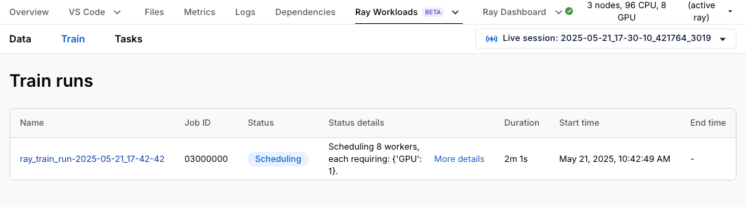
If you are using an Anyscale Workspace, go to the Ray Train dashboard to analyze your distributed training job. Click Ray Workloads and then Ray Train, which shows a list of all the training runs you have kicked off.
Clicking the run displays an overview page that shows logs from the controller, which is the process that coordinates your entire Ray Train job, as well as information about the 8 training workers.
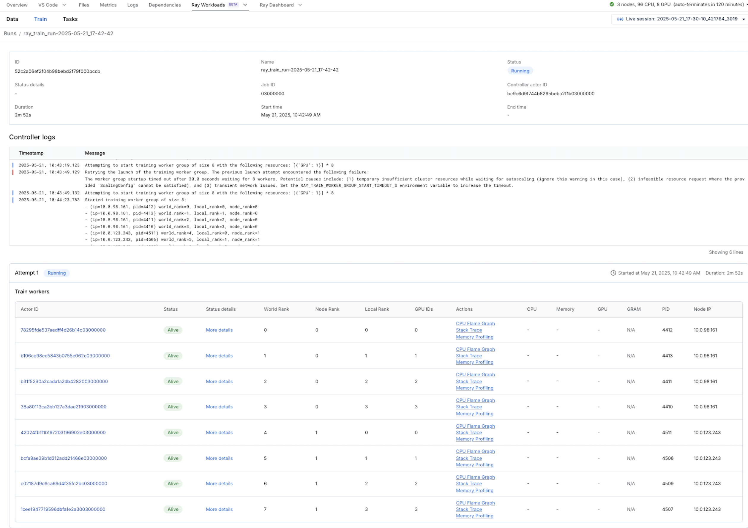
Click an individual worker for a more detailed worker page.

If your worker is still alive, you can click CPU Flame Graph, Stack Trace, or Memory Profiling links in the overall run page or the individual worker page. Clicking CPU Flame Graph profiles your run with py-spy for 5 seconds and shows a CPU flame graph. Clicking Stack Trace shows the current stack trace of your job, which is useful for debugging hanging jobs. Finally, clicking Memory Profiling profiles your run with memray for 5 seconds and shows a memory flame graph.
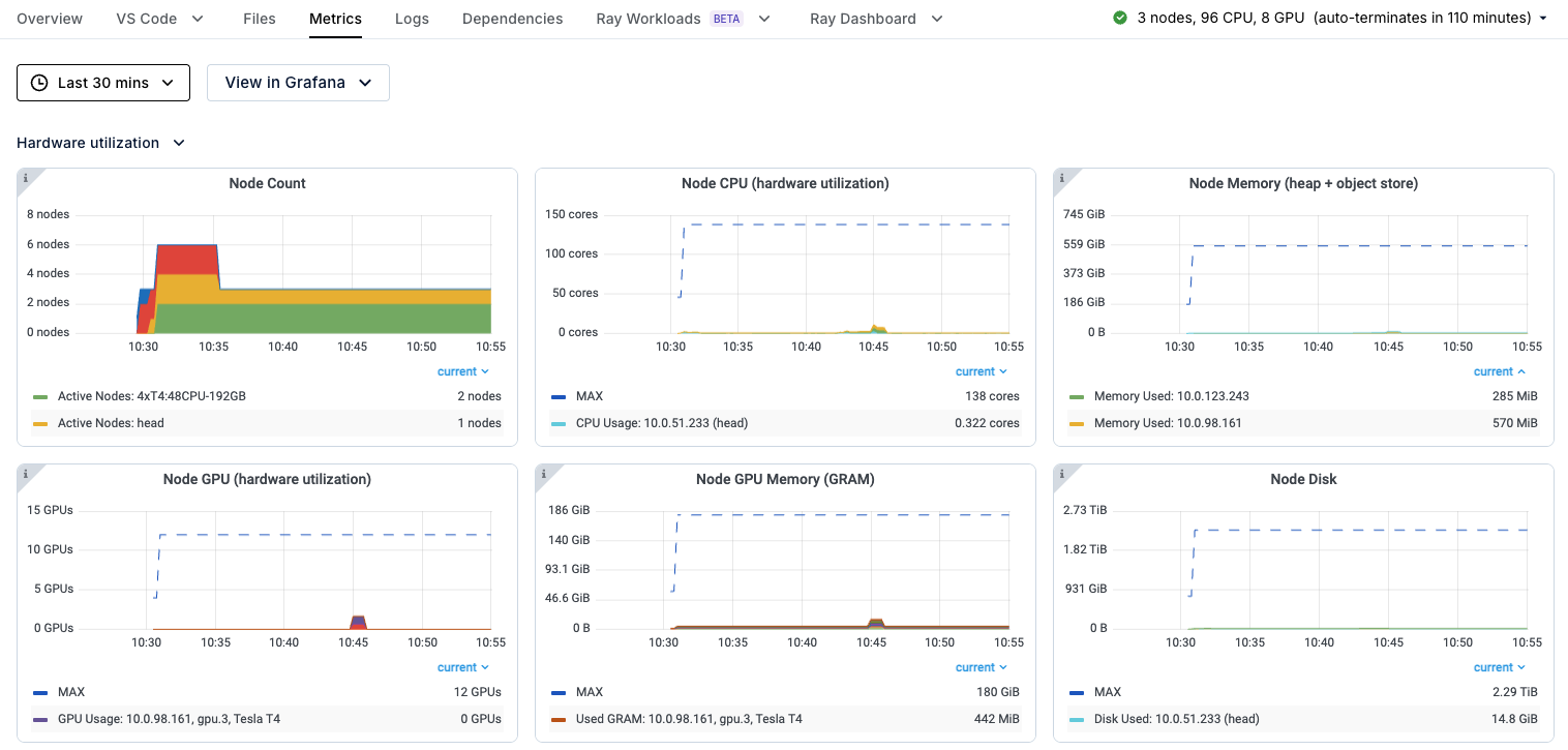
You can also click the Metrics tab on the navigation bar to view useful stats about the cluster, such as GPU utilization and metrics about Ray actors and tasks.
Step 3: Scale data ingest separately from training with Ray Data#
Modify this example to load data with Ray Data instead of the native PyTorch DataLoader. With a few modifications, you can scale data preprocessing and training separately. For example, you can do the former with a pool of CPU workers and the latter with a pool of GPU workers. See How does Ray Data compare to other solutions for offline inference? for a comparison between Ray Data and PyTorch data loading.
First, create Ray Data Datasets from S3 data and inspect their schemas.
import ray.data

import numpy as np

STORAGE_PATH = "s3://ray-example-data/cifar10-parquet"
train_dataset = ray.data.read_parquet(f'{STORAGE_PATH}/train')
test_dataset = ray.data.read_parquet(f'{STORAGE_PATH}/test')
train_dataset.schema()
test_dataset.schema()
Next, use Ray Data to transform the data. Note that both loading and transformation happen lazily, which means that only the training workers materialize the data.
def transform_cifar(row: Dict[str, np.ndarray]) -> Dict[str, np.ndarray]:
    # Define the torchvision transform.
    transform = transforms.Compose([ToTensor(), Normalize((0.5, 0.5, 0.5), (0.5, 0.5, 0.5))])
    row["image"] = transform(row["image"])
    return row

train_dataset = train_dataset.map(transform_cifar)
test_dataset = test_dataset.map(transform_cifar)
Next, modify the training function you wrote earlier. Every difference from the previous script is highlighted and explained with a numbered comment; for example, “[1].”
def train_func_per_worker(config: Dict):
    lr = config["lr"]
    epochs = config["epochs"]
    batch_size = config["batch_size_per_worker"]


    # [1] Prepare `Dataloader` for distributed training.
    # The get_dataset_shard method gets the associated dataset shard to pass to the
    # TorchTrainer constructor in the next code block.
    # The iter_torch_batches method lazily shards the dataset among workers.
    # =============================================================================
    train_data_shard = ray.train.get_dataset_shard("train")
    valid_data_shard = ray.train.get_dataset_shard("valid")
    train_dataloader = train_data_shard.iter_torch_batches(batch_size=batch_size)
    valid_dataloader = valid_data_shard.iter_torch_batches(batch_size=batch_size)

    model = VisionTransformer(
        image_size=32,   # CIFAR-10 image size is 32x32
        patch_size=4,    # Patch size is 4x4
        num_layers=12,   # Number of transformer layers
        num_heads=8,     # Number of attention heads
        hidden_dim=384,  # Hidden size (can be adjusted)
        mlp_dim=768,     # MLP dimension (can be adjusted)
        num_classes=10   # CIFAR-10 has 10 classes
    )

    model = ray.train.torch.prepare_model(model)

    loss_fn = nn.CrossEntropyLoss()
    optimizer = torch.optim.AdamW(model.parameters(), lr=lr, weight_decay=1e-2)

    # Model training loop.
    for epoch in range(epochs):
        model.train()
        for batch in tqdm(train_dataloader, desc=f"Train Epoch {epoch}"):
            X, y = batch['image'], batch['label']
            pred = model(X)
            loss = loss_fn(pred, y)

            optimizer.zero_grad()
            loss.backward()
            optimizer.step()

        model.eval()
        valid_loss, num_correct, num_total, num_batches = 0, 0, 0, 0
        with torch.no_grad():
            for batch in tqdm(valid_dataloader, desc=f"Valid Epoch {epoch}"):
                # [2] Each Ray Data batch is a dict so you must access the
                # underlying data using the appropriate keys.
                # =======================================================
                X, y = batch['image'], batch['label']
                pred = model(X)
                loss = loss_fn(pred, y)

                valid_loss += loss.item()
                num_total += y.shape[0]
                num_batches += 1
                num_correct += (pred.argmax(1) == y).sum().item()

        valid_loss /= num_batches
        accuracy = num_correct / num_total

        with tempfile.TemporaryDirectory() as temp_checkpoint_dir:
            torch.save(
                model.module.state_dict(),
                os.path.join(temp_checkpoint_dir, "model.pt")
            )
            ray.train.report(
                metrics={"loss": valid_loss, "accuracy": accuracy},
                checkpoint=ray.train.Checkpoint.from_directory(temp_checkpoint_dir),
            )
            if ray.train.get_context().get_world_rank() == 0:
                print({"epoch_num": epoch, "loss": valid_loss, "accuracy": accuracy})
Finally, run the training function with the Ray Data Dataset on the Ray Cluster with 8 GPU workers.
def train_cifar_10(num_workers, use_gpu):
    global_batch_size = 512

    train_config = {
        "lr": 1e-3,
        "epochs": 1,
        "batch_size_per_worker": global_batch_size // num_workers,
    }

    # Configure computation resources.
    scaling_config = ScalingConfig(num_workers=num_workers, use_gpu=use_gpu)
    run_config = RunConfig(
        storage_path="/mnt/cluster_storage",
        name=f"train_data_run-{uuid.uuid4().hex}",
    )

    # Initialize a Ray TorchTrainer.
    trainer = TorchTrainer(
        train_loop_per_worker=train_func_per_worker,
        # [1] With Ray Data you pass the Dataset directly to the Trainer.
        # ==============================================================
        datasets={"train": train_dataset, "valid": test_dataset},
        train_loop_config=train_config,
        scaling_config=scaling_config,
        run_config=run_config,
    )

    result = trainer.fit()
    print(f"Training result: {result}")

if __name__ == "__main__":
    train_cifar_10(num_workers=8, use_gpu=True)
Once again your training run should take around 1 minute with similar accuracy. There aren’t big performance wins with Ray Data on this example due to the small size of the dataset; for more interesting benchmarking information see this blog post. The main advantage of Ray Data is that it allows you to stream data across heterogeneous compute, maximizing GPU utilization while minimizing RAM usage.
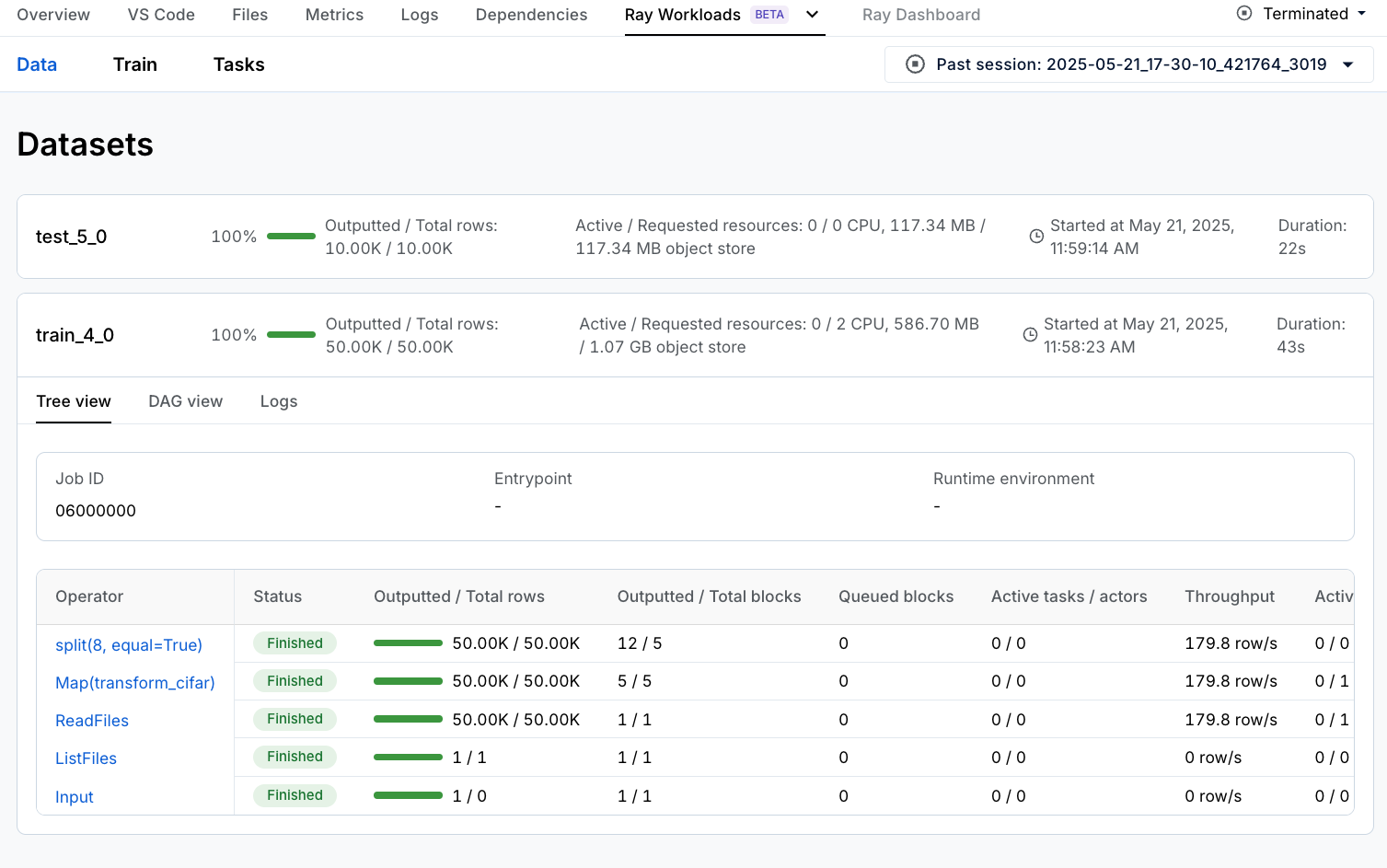
If you are using an Anyscale Workspace, in addition to the Ray Train and Metrics dashboards you saw in the previous section, you can also view the Ray Data dashboard by clicking Ray Workloads and then Data where you can view the throughput and status of each Ray Data operator.
Summary#
In this notebook, you:
Trained a PyTorch VisionTransformer model on a Ray Cluster with multiple GPU workers with Ray Train and Ray Data
Verified that speed improved without affecting accuracy
Gained insight into your distributed training and data preprocessing workloads with various dashboards