Note

Ray 2.10.0 introduces the alpha stage of RLlib’s “new API stack”. The team is currently transitioning algorithms, example scripts, and documentation to the new code base throughout the subsequent minor releases leading up to Ray 3.0.

See here for more details on how to activate and use the new API stack.

Algorithms#

Overview#

The following table is an overview of all available algorithms in RLlib. Note that all of them support multi-GPU training on a single (GPU) node in Ray (open-source) () as well as multi-GPU training on multi-node (GPU) clusters when using the Anyscale platform ().

Algorithm	Single- and Multi-agent	Multi-GPU (multi-node)	Action Spaces
On-Policy
PPO (Proximal Policy Optimization)
Off-Policy
DQN/Rainbow (Deep Q Networks)
SAC (Soft Actor Critic)
High-throughput on- and off policy
APPO (Asynchronous Proximal Policy Optimization)
IMPALA (Importance Weighted Actor-Learner Architecture)
Model-based RL
DreamerV3
Offline RL and Imitation Learning
BC (Behavior Cloning)
MARWIL (Monotonic Advantage Re-Weighted Imitation Learning)
Algorithm Extensions and -Plugins
Curiosity-driven Exploration by Self-supervised Prediction

On-policy#

Proximal Policy Optimization (PPO)#

[paper] [implementation]

../_images/ppo-architecture.svg — **PPO architecture:** In a training iteration, PPO performs three major steps: 1. Sampling a set of episodes or episode fragments 1. Converting these into a train batch and updating the model using a clipped objective and multiple SGD passes over this batch 1. Synching the weights from the Learners back to the EnvRunners PPO scales out on both axes, supporting multiple EnvRunners for sample collection and multiple GPU- or CPU-based Learners for updating the model.#

Tuned examples: Pong-v5, CartPole-v1. Pendulum-v1.

PPO-specific configs (see also common configs):

class ray.rllib.algorithms.ppo.ppo.PPOConfig(algo_class=None)[source]#

Defines a configuration class from which a PPO Algorithm can be built.

from ray.rllib.algorithms.ppo import PPOConfig

config = PPOConfig()
config.environment("CartPole-v1")
config.env_runners(num_env_runners=1)
config.training(
    gamma=0.9, lr=0.01, kl_coeff=0.3, train_batch_size_per_learner=256
)

# Build a Algorithm object from the config and run 1 training iteration.
algo = config.build()
algo.train()

from ray.rllib.algorithms.ppo import PPOConfig
from ray import air
from ray import tune

config = (
    PPOConfig()
    # Set the config object's env.
    .environment(env="CartPole-v1")
    # Update the config object's training parameters.
    .training(
        lr=0.001, clip_param=0.2
    )
)

tune.Tuner(
    "PPO",
    run_config=air.RunConfig(stop={"training_iteration": 1}),
    param_space=config,
).fit()

training(*, use_critic: bool | None = <ray.rllib.utils.from_config._NotProvided object>, use_gae: bool | None = <ray.rllib.utils.from_config._NotProvided object>, lambda_: float | None = <ray.rllib.utils.from_config._NotProvided object>, use_kl_loss: bool | None = <ray.rllib.utils.from_config._NotProvided object>, kl_coeff: float | None = <ray.rllib.utils.from_config._NotProvided object>, kl_target: float | None = <ray.rllib.utils.from_config._NotProvided object>, vf_loss_coeff: float | None = <ray.rllib.utils.from_config._NotProvided object>, entropy_coeff: float | None = <ray.rllib.utils.from_config._NotProvided object>, entropy_coeff_schedule: ~typing.List[~typing.List[int | float]] | None = <ray.rllib.utils.from_config._NotProvided object>, clip_param: float | None = <ray.rllib.utils.from_config._NotProvided object>, vf_clip_param: float | None = <ray.rllib.utils.from_config._NotProvided object>, grad_clip: float | None = <ray.rllib.utils.from_config._NotProvided object>, lr_schedule: ~typing.List[~typing.List[int | float]] | None = <ray.rllib.utils.from_config._NotProvided object>, vf_share_layers=-1, **kwargs) → PPOConfig[source]#

Sets the training related configuration.

Parameters:

use_critic – Should use a critic as a baseline (otherwise don’t use value baseline; required for using GAE).
use_gae – If true, use the Generalized Advantage Estimator (GAE) with a value function, see https://arxiv.org/pdf/1506.02438.pdf.
lambda – The lambda parameter for General Advantage Estimation (GAE). Defines the exponential weight used between actually measured rewards vs value function estimates over multiple time steps. Specifically, lambda_ balances short-term, low-variance estimates against long-term, high-variance returns. A lambda_ of 0.0 makes the GAE rely only on immediate rewards (and vf predictions from there on, reducing variance, but increasing bias), while a lambda_ of 1.0 only incorporates vf predictions at the truncation points of the given episodes or episode chunks (reducing bias but increasing variance).
use_kl_loss – Whether to use the KL-term in the loss function.
kl_coeff – Initial coefficient for KL divergence.
kl_target – Target value for KL divergence.
vf_loss_coeff – Coefficient of the value function loss. IMPORTANT: you must tune this if you set vf_share_layers=True inside your model’s config.
entropy_coeff – The entropy coefficient (float) or entropy coefficient schedule in the format of [[timestep, coeff-value], [timestep, coeff-value], …] In case of a schedule, intermediary timesteps will be assigned to linearly interpolated coefficient values. A schedule config’s first entry must start with timestep 0, i.e.: [[0, initial_value], […]].
clip_param – The PPO clip parameter.
vf_clip_param – Clip param for the value function. Note that this is sensitive to the scale of the rewards. If your expected V is large, increase this.
grad_clip – If specified, clip the global norm of gradients by this amount.

Returns:

This updated AlgorithmConfig object.

Off-Policy#

Deep Q Networks (DQN, Rainbow, Parametric DQN)#

[paper] [implementation]

../_images/dqn-architecture.svg — **DQN architecture:** DQN uses a replay buffer to temporarily store episode samples that RLlib collects from the environment. Throughout different training iterations, these episodes and episode fragments are re-sampled from the buffer and re-used for updating the model, before eventually being discarded when the buffer has reached capacity and new samples keep coming in (FIFO). This reuse of training data makes DQN very sample-efficient and off-policy. DQN scales out on both axes, supporting multiple EnvRunners for sample collection and multiple GPU- or CPU-based Learners for updating the model.#

All of the DQN improvements evaluated in Rainbow are available, though not all are enabled by default. See also how to use parametric-actions in DQN.

Tuned examples: PongDeterministic-v4, Rainbow configuration, {BeamRider,Breakout,Qbert,SpaceInvaders}NoFrameskip-v4, with Dueling and Double-Q, with Distributional DQN.

Hint

For a complete rainbow setup, make the following changes to the default DQN config: "n_step": [between 1 and 10], "noisy": True, "num_atoms": [more than 1], "v_min": -10.0, "v_max": 10.0 (set v_min and v_max according to your expected range of returns).

DQN-specific configs (see also common configs):

class ray.rllib.algorithms.dqn.dqn.DQNConfig(algo_class=None)[source]#

Defines a configuration class from which a DQN Algorithm can be built.

from ray.rllib.algorithms.dqn.dqn import DQNConfig

config = (
    DQNConfig()
    .environment("CartPole-v1")
    .training(replay_buffer_config={
        "type": "PrioritizedEpisodeReplayBuffer",
        "capacity": 60000,
        "alpha": 0.5,
        "beta": 0.5,
    })
    .env_runners(num_env_runners=1)
)
algo = config.build()
algo.train()
algo.stop()

from ray.rllib.algorithms.dqn.dqn import DQNConfig
from ray import air
from ray import tune

config = (
    DQNConfig()
    .environment("CartPole-v1")
    .training(
        num_atoms=tune.grid_search([1,])
    )
)
tune.Tuner(
    "DQN",
    run_config=air.RunConfig(stop={"training_iteration":1}),
    param_space=config,
).fit()

training(*, target_network_update_freq: int | None = <ray.rllib.utils.from_config._NotProvided object>, replay_buffer_config: dict | None = <ray.rllib.utils.from_config._NotProvided object>, store_buffer_in_checkpoints: bool | None = <ray.rllib.utils.from_config._NotProvided object>, lr_schedule: ~typing.List[~typing.List[int | float]] | None = <ray.rllib.utils.from_config._NotProvided object>, epsilon: float | ~typing.List[~typing.List[int | float]] | ~typing.List[~typing.Tuple[int, int | float]] | None = <ray.rllib.utils.from_config._NotProvided object>, adam_epsilon: float | None = <ray.rllib.utils.from_config._NotProvided object>, grad_clip: int | None = <ray.rllib.utils.from_config._NotProvided object>, num_steps_sampled_before_learning_starts: int | None = <ray.rllib.utils.from_config._NotProvided object>, tau: float | None = <ray.rllib.utils.from_config._NotProvided object>, num_atoms: int | None = <ray.rllib.utils.from_config._NotProvided object>, v_min: float | None = <ray.rllib.utils.from_config._NotProvided object>, v_max: float | None = <ray.rllib.utils.from_config._NotProvided object>, noisy: bool | None = <ray.rllib.utils.from_config._NotProvided object>, sigma0: float | None = <ray.rllib.utils.from_config._NotProvided object>, dueling: bool | None = <ray.rllib.utils.from_config._NotProvided object>, hiddens: int | None = <ray.rllib.utils.from_config._NotProvided object>, double_q: bool | None = <ray.rllib.utils.from_config._NotProvided object>, n_step: int | ~typing.Tuple[int, int] | None = <ray.rllib.utils.from_config._NotProvided object>, before_learn_on_batch: ~typing.Callable[[~typing.Type[~ray.rllib.policy.sample_batch.MultiAgentBatch], ~typing.List[~typing.Type[~ray.rllib.policy.policy.Policy]], ~typing.Type[int]], ~typing.Type[~ray.rllib.policy.sample_batch.MultiAgentBatch]] = <ray.rllib.utils.from_config._NotProvided object>, training_intensity: float | None = <ray.rllib.utils.from_config._NotProvided object>, td_error_loss_fn: str | None = <ray.rllib.utils.from_config._NotProvided object>, categorical_distribution_temperature: float | None = <ray.rllib.utils.from_config._NotProvided object>, **kwargs) → DQNConfig[source]#

Sets the training related configuration.

Parameters:

target_network_update_freq – Update the target network every target_network_update_freq sample steps.
replay_buffer_config – Replay buffer config. Examples: { “_enable_replay_buffer_api”: True, “type”: “MultiAgentReplayBuffer”, “capacity”: 50000, “replay_sequence_length”: 1, } - OR - { “_enable_replay_buffer_api”: True, “type”: “MultiAgentPrioritizedReplayBuffer”, “capacity”: 50000, “prioritized_replay_alpha”: 0.6, “prioritized_replay_beta”: 0.4, “prioritized_replay_eps”: 1e-6, “replay_sequence_length”: 1, } - Where - prioritized_replay_alpha: Alpha parameter controls the degree of prioritization in the buffer. In other words, when a buffer sample has a higher temporal-difference error, with how much more probability should it drawn to use to update the parametrized Q-network. 0.0 corresponds to uniform probability. Setting much above 1.0 may quickly result as the sampling distribution could become heavily “pointy” with low entropy. prioritized_replay_beta: Beta parameter controls the degree of importance sampling which suppresses the influence of gradient updates from samples that have higher probability of being sampled via alpha parameter and the temporal-difference error. prioritized_replay_eps: Epsilon parameter sets the baseline probability for sampling so that when the temporal-difference error of a sample is zero, there is still a chance of drawing the sample.
store_buffer_in_checkpoints – Set this to True, if you want the contents of your buffer(s) to be stored in any saved checkpoints as well. Warnings will be created if: - This is True AND restoring from a checkpoint that contains no buffer data. - This is False AND restoring from a checkpoint that does contain buffer data.
epsilon – Epsilon exploration schedule. In the format of [[timestep, value], [timestep, value], …]. A schedule must start from timestep 0.
adam_epsilon – Adam optimizer’s epsilon hyper parameter.
grad_clip – If not None, clip gradients during optimization at this value.
num_steps_sampled_before_learning_starts – Number of timesteps to collect from rollout workers before we start sampling from replay buffers for learning. Whether we count this in agent steps or environment steps depends on config.multi_agent(count_steps_by=..).
tau – Update the target by au * policy + (1- au) * target_policy.
num_atoms – Number of atoms for representing the distribution of return. When this is greater than 1, distributional Q-learning is used.
v_min – Minimum value estimation
v_max – Maximum value estimation
noisy – Whether to use noisy network to aid exploration. This adds parametric noise to the model weights.
sigma0 – Control the initial parameter noise for noisy nets.
dueling – Whether to use dueling DQN.
hiddens – Dense-layer setup for each the advantage branch and the value branch
double_q – Whether to use double DQN.
n_step – N-step target updates. If >1, sars’ tuples in trajectories will be postprocessed to become sa[discounted sum of R][s t+n] tuples. An integer will be interpreted as a fixed n-step value. If a tuple of 2 ints is provided here, the n-step value will be drawn for each sample(!) in the train batch from a uniform distribution over the closed interval defined by [n_step[0], n_step[1]].
before_learn_on_batch – Callback to run before learning on a multi-agent batch of experiences.
training_intensity – The intensity with which to update the model (vs collecting samples from the env). If None, uses “natural” values of: train_batch_size / (rollout_fragment_length x num_env_runners x num_envs_per_env_runner). If not None, will make sure that the ratio between timesteps inserted into and sampled from the buffer matches the given values. Example: training_intensity=1000.0 train_batch_size=250 rollout_fragment_length=1 num_env_runners=1 (or 0) num_envs_per_env_runner=1 -> natural value = 250 / 1 = 250.0 -> will make sure that replay+train op will be executed 4x asoften as rollout+insert op (4 * 250 = 1000). See: rllib/algorithms/dqn/dqn.py::calculate_rr_weights for further details.
td_error_loss_fn – “huber” or “mse”. loss function for calculating TD error when num_atoms is 1. Note that if num_atoms is > 1, this parameter is simply ignored, and softmax cross entropy loss will be used.
categorical_distribution_temperature – Set the temperature parameter used by Categorical action distribution. A valid temperature is in the range of [0, 1]. Note that this mostly affects evaluation since TD error uses argmax for return calculation.

Returns:

This updated AlgorithmConfig object.

Soft Actor Critic (SAC)#

[original paper], [follow up paper], [implementation].

../_images/sac-architecture.svg — **SAC architecture:** SAC uses a replay buffer to temporarily store episode samples that RLlib collects from the environment. Throughout different training iterations, these episodes and episode fragments are re-sampled from the buffer and re-used for updating the model, before eventually being discarded when the buffer has reached capacity and new samples keep coming in (FIFO). This reuse of training data makes DQN very sample-efficient and off-policy. SAC scales out on both axes, supporting multiple EnvRunners for sample collection and multiple GPU- or CPU-based Learners for updating the model.#

Tuned examples: Pendulum-v1, HalfCheetah-v3,

SAC-specific configs (see also common configs):

class ray.rllib.algorithms.sac.sac.SACConfig(algo_class=None)[source]#

Defines a configuration class from which an SAC Algorithm can be built.

config = (
    SACConfig()
    .environment("Pendulum-v1")
    .env_runners(num_env_runners=1)
    .training(
        gamma=0.9,
        actor_lr=0.001,
        critic_lr=0.002,
        train_batch_size_per_learner=32,
    )
)
# Build the SAC algo object from the config and run 1 training iteration.
algo = config.build()
algo.train()

training(*, twin_q: bool | None = <ray.rllib.utils.from_config._NotProvided object>, q_model_config: ~typing.Dict[str, ~typing.Any] | None = <ray.rllib.utils.from_config._NotProvided object>, policy_model_config: ~typing.Dict[str, ~typing.Any] | None = <ray.rllib.utils.from_config._NotProvided object>, tau: float | None = <ray.rllib.utils.from_config._NotProvided object>, initial_alpha: float | None = <ray.rllib.utils.from_config._NotProvided object>, target_entropy: str | float | None = <ray.rllib.utils.from_config._NotProvided object>, n_step: int | ~typing.Tuple[int, int] | None = <ray.rllib.utils.from_config._NotProvided object>, store_buffer_in_checkpoints: bool | None = <ray.rllib.utils.from_config._NotProvided object>, replay_buffer_config: ~typing.Dict[str, ~typing.Any] | None = <ray.rllib.utils.from_config._NotProvided object>, training_intensity: float | None = <ray.rllib.utils.from_config._NotProvided object>, clip_actions: bool | None = <ray.rllib.utils.from_config._NotProvided object>, grad_clip: float | None = <ray.rllib.utils.from_config._NotProvided object>, optimization_config: ~typing.Dict[str, ~typing.Any] | None = <ray.rllib.utils.from_config._NotProvided object>, actor_lr: float | ~typing.List[~typing.List[int | float]] | ~typing.List[~typing.Tuple[int, int | float]] | None = <ray.rllib.utils.from_config._NotProvided object>, critic_lr: float | ~typing.List[~typing.List[int | float]] | ~typing.List[~typing.Tuple[int, int | float]] | None = <ray.rllib.utils.from_config._NotProvided object>, alpha_lr: float | ~typing.List[~typing.List[int | float]] | ~typing.List[~typing.Tuple[int, int | float]] | None = <ray.rllib.utils.from_config._NotProvided object>, target_network_update_freq: int | None = <ray.rllib.utils.from_config._NotProvided object>, _deterministic_loss: bool | None = <ray.rllib.utils.from_config._NotProvided object>, _use_beta_distribution: bool | None = <ray.rllib.utils.from_config._NotProvided object>, num_steps_sampled_before_learning_starts: int | None = <ray.rllib.utils.from_config._NotProvided object>, **kwargs) → SACConfig[source]#

Sets the training related configuration.

Parameters:

twin_q – Use two Q-networks (instead of one) for action-value estimation. Note: Each Q-network will have its own target network.
q_model_config – Model configs for the Q network(s). These will override MODEL_DEFAULTS. This is treated just as the top-level model dict in setting up the Q-network(s) (2 if twin_q=True). That means, you can do for different observation spaces: obs=Box(1D) -> Tuple(Box(1D) + Action) -> concat -> post_fcnet obs=Box(3D) -> Tuple(Box(3D) + Action) -> vision-net -> concat w/ action -> post_fcnet obs=Tuple(Box(1D), Box(3D)) -> Tuple(Box(1D), Box(3D), Action) -> vision-net -> concat w/ Box(1D) and action -> post_fcnet You can also have SAC use your custom_model as Q-model(s), by simply specifying the custom_model sub-key in below dict (just like you would do in the top-level model dict.
policy_model_config – Model options for the policy function (see q_model_config above for details). The difference to q_model_config above is that no action concat’ing is performed before the post_fcnet stack.
tau – Update the target by au * policy + (1- au) * target_policy.
initial_alpha – Initial value to use for the entropy weight alpha.
target_entropy – Target entropy lower bound. If “auto”, will be set to -|A| (e.g. -2.0 for Discrete(2), -3.0 for Box(shape=(3,))). This is the inverse of reward scale, and will be optimized automatically.
n_step – N-step target updates. If >1, sars’ tuples in trajectories will be postprocessed to become sa[discounted sum of R][s t+n] tuples. An integer will be interpreted as a fixed n-step value. If a tuple of 2 ints is provided here, the n-step value will be drawn for each sample(!) in the train batch from a uniform distribution over the closed interval defined by [n_step[0], n_step[1]].
store_buffer_in_checkpoints – Set this to True, if you want the contents of your buffer(s) to be stored in any saved checkpoints as well. Warnings will be created if: - This is True AND restoring from a checkpoint that contains no buffer data. - This is False AND restoring from a checkpoint that does contain buffer data.
replay_buffer_config – Replay buffer config. Examples: { “_enable_replay_buffer_api”: True, “type”: “MultiAgentReplayBuffer”, “capacity”: 50000, “replay_batch_size”: 32, “replay_sequence_length”: 1, } - OR - { “_enable_replay_buffer_api”: True, “type”: “MultiAgentPrioritizedReplayBuffer”, “capacity”: 50000, “prioritized_replay_alpha”: 0.6, “prioritized_replay_beta”: 0.4, “prioritized_replay_eps”: 1e-6, “replay_sequence_length”: 1, } - Where - prioritized_replay_alpha: Alpha parameter controls the degree of prioritization in the buffer. In other words, when a buffer sample has a higher temporal-difference error, with how much more probability should it drawn to use to update the parametrized Q-network. 0.0 corresponds to uniform probability. Setting much above 1.0 may quickly result as the sampling distribution could become heavily “pointy” with low entropy. prioritized_replay_beta: Beta parameter controls the degree of importance sampling which suppresses the influence of gradient updates from samples that have higher probability of being sampled via alpha parameter and the temporal-difference error. prioritized_replay_eps: Epsilon parameter sets the baseline probability for sampling so that when the temporal-difference error of a sample is zero, there is still a chance of drawing the sample.
training_intensity – The intensity with which to update the model (vs collecting samples from the env). If None, uses “natural” values of: train_batch_size / (rollout_fragment_length x num_env_runners x num_envs_per_env_runner). If not None, will make sure that the ratio between timesteps inserted into and sampled from th buffer matches the given values. Example: training_intensity=1000.0 train_batch_size=250 rollout_fragment_length=1 num_env_runners=1 (or 0) num_envs_per_env_runner=1 -> natural value = 250 / 1 = 250.0 -> will make sure that replay+train op will be executed 4x asoften as rollout+insert op (4 * 250 = 1000). See: rllib/algorithms/dqn/dqn.py::calculate_rr_weights for further details.
clip_actions – Whether to clip actions. If actions are already normalized, this should be set to False.
grad_clip – If not None, clip gradients during optimization at this value.
optimization_config – Config dict for optimization. Set the supported keys actor_learning_rate, critic_learning_rate, and entropy_learning_rate in here.
actor_lr – The learning rate (float) or learning rate schedule for the policy in the format of [[timestep, lr-value], [timestep, lr-value], …] In case of a schedule, intermediary timesteps will be assigned to linearly interpolated learning rate values. A schedule config’s first entry must start with timestep 0, i.e.: [[0, initial_value], […]]. Note: It is common practice (two-timescale approach) to use a smaller learning rate for the policy than for the critic to ensure that the critic gives adequate values for improving the policy. Note: If you require a) more than one optimizer (per RLModule), b) optimizer types that are not Adam, c) a learning rate schedule that is not a linearly interpolated, piecewise schedule as described above, or d) specifying c’tor arguments of the optimizer that are not the learning rate (e.g. Adam’s epsilon), then you must override your Learner’s configure_optimizer_for_module() method and handle lr-scheduling yourself. The default value is 3e-5, one decimal less than the respective learning rate of the critic (see critic_lr).
critic_lr – The learning rate (float) or learning rate schedule for the critic in the format of [[timestep, lr-value], [timestep, lr-value], …] In case of a schedule, intermediary timesteps will be assigned to linearly interpolated learning rate values. A schedule config’s first entry must start with timestep 0, i.e.: [[0, initial_value], […]]. Note: It is common practice (two-timescale approach) to use a smaller learning rate for the policy than for the critic to ensure that the critic gives adequate values for improving the policy. Note: If you require a) more than one optimizer (per RLModule), b) optimizer types that are not Adam, c) a learning rate schedule that is not a linearly interpolated, piecewise schedule as described above, or d) specifying c’tor arguments of the optimizer that are not the learning rate (e.g. Adam’s epsilon), then you must override your Learner’s configure_optimizer_for_module() method and handle lr-scheduling yourself. The default value is 3e-4, one decimal higher than the respective learning rate of the actor (policy) (see actor_lr).
alpha_lr – The learning rate (float) or learning rate schedule for the hyperparameter alpha in the format of [[timestep, lr-value], [timestep, lr-value], …] In case of a schedule, intermediary timesteps will be assigned to linearly interpolated learning rate values. A schedule config’s first entry must start with timestep 0, i.e.: [[0, initial_value], […]]. Note: If you require a) more than one optimizer (per RLModule), b) optimizer types that are not Adam, c) a learning rate schedule that is not a linearly interpolated, piecewise schedule as described above, or d) specifying c’tor arguments of the optimizer that are not the learning rate (e.g. Adam’s epsilon), then you must override your Learner’s configure_optimizer_for_module() method and handle lr-scheduling yourself. The default value is 3e-4, identical to the critic learning rate (lr).
target_network_update_freq – Update the target network every target_network_update_freq steps.
_deterministic_loss – Whether the loss should be calculated deterministically (w/o the stochastic action sampling step). True only useful for continuous actions and for debugging.
_use_beta_distribution – Use a Beta-distribution instead of a SquashedGaussian for bounded, continuous action spaces (not recommended; for debugging only).

Returns:

This updated AlgorithmConfig object.

High-Throughput On- and Off-Policy#

Asynchronous Proximal Policy Optimization (APPO)#

Tip

APPO was originally published under the name “IMPACT”. RLlib’s APPO exactly matches the algorithm described in the paper.

[paper] [implementation]

../_images/appo-architecture.svg — **APPO architecture:** APPO is an asynchronous variant of Proximal Policy Optimization (PPO) based on the IMPALA architecture, but using a surrogate policy loss with clipping, allowing for multiple SGD passes per collected train batch. In a training iteration, APPO requests samples from all EnvRunners asynchronously and the collected episode samples are returned to the main algorithm process as Ray references rather than actual objects available on the local process. APPO then passes these episode references to the Learners for asynchronous updates of the model. RLlib doesn’t always synch back the weights to the EnvRunners right after a new model version is available. To account for the EnvRunners being off-policy, APPO uses a procedure called v-trace, described in the IMPALA paper. APPO scales out on both axes, supporting multiple EnvRunners for sample collection and multiple GPU- or CPU-based Learners for updating the model.#

Tuned examples: Pong-v5 HalfCheetah-v4

APPO-specific configs (see also common configs):

class ray.rllib.algorithms.appo.appo.APPOConfig(algo_class=None)[source]#

Defines a configuration class from which an APPO Algorithm can be built.

from ray.rllib.algorithms.appo import APPOConfig
config = (
    APPOConfig()
    .training(lr=0.01, grad_clip=30.0, train_batch_size_per_learner=50)
)
config = config.learners(num_learners=1)
config = config.env_runners(num_env_runners=1)
config = config.environment("CartPole-v1")

# Build an Algorithm object from the config and run 1 training iteration.
algo = config.build()
algo.train()
del algo

from ray.rllib.algorithms.appo import APPOConfig
from ray import air
from ray import tune

config = APPOConfig()
# Update the config object.
config = config.training(lr=tune.grid_search([0.001,]))
# Set the config object's env.
config = config.environment(env="CartPole-v1")
# Use to_dict() to get the old-style python config dict when running with tune.
tune.Tuner(
    "APPO",
    run_config=air.RunConfig(
        stop={"training_iteration": 1},
        verbose=0,
    ),
    param_space=config.to_dict(),

).fit()

training(*, vtrace: bool | None = <ray.rllib.utils.from_config._NotProvided object>, use_gae: bool | None = <ray.rllib.utils.from_config._NotProvided object>, lambda_: float | None = <ray.rllib.utils.from_config._NotProvided object>, clip_param: float | None = <ray.rllib.utils.from_config._NotProvided object>, use_kl_loss: bool | None = <ray.rllib.utils.from_config._NotProvided object>, kl_coeff: float | None = <ray.rllib.utils.from_config._NotProvided object>, kl_target: float | None = <ray.rllib.utils.from_config._NotProvided object>, target_network_update_freq: int | None = <ray.rllib.utils.from_config._NotProvided object>, tau: float | None = <ray.rllib.utils.from_config._NotProvided object>, target_worker_clipping: float | None = <ray.rllib.utils.from_config._NotProvided object>, circular_buffer_num_batches: int | None = <ray.rllib.utils.from_config._NotProvided object>, circular_buffer_iterations_per_batch: int | None = <ray.rllib.utils.from_config._NotProvided object>, target_update_frequency=-1, use_critic=-1, **kwargs) → APPOConfig[source]#

Sets the training related configuration.

Parameters:

vtrace – Whether to use V-trace weighted advantages. If false, PPO GAE advantages will be used instead.
use_gae – If true, use the Generalized Advantage Estimator (GAE) with a value function, see https://arxiv.org/pdf/1506.02438.pdf. Only applies if vtrace=False.
lambda – GAE (lambda) parameter.
clip_param – PPO surrogate slipping parameter.
use_kl_loss – Whether to use the KL-term in the loss function.
kl_coeff – Coefficient for weighting the KL-loss term.
kl_target – Target term for the KL-term to reach (via adjusting the kl_coeff automatically).
target_network_update_freq – NOTE: This parameter is only applicable on the new API stack. The frequency with which to update the target policy network from the main trained policy network. The metric used is NUM_ENV_STEPS_TRAINED_LIFETIME and the unit is n (see [1] 4.1.1), where: n = [circular_buffer_num_batches (N)] * [circular_buffer_iterations_per_batch (K)] * [train batch size] For example, if you set target_network_update_freq=2, and N=4, K=2, and train_batch_size_per_learner=500, then the target net is updated every 2*4*2*500=8000 trained env steps (every 16 batch updates on each learner). The authors in [1] suggests that this setting is robust to a range of choices (try values between 0.125 and 4).
target_network_update_freq – The frequency to update the target policy and tune the kl loss coefficients that are used during training. After setting this parameter, the algorithm waits for at least target_network_update_freq number of environment samples to be trained on before updating the target networks and tune the kl loss coefficients. NOTE: This parameter is only applicable when using the Learner API (enable_rl_module_and_learner=True).
tau – The factor by which to update the target policy network towards the current policy network. Can range between 0 and 1. e.g. updated_param = tau * current_param + (1 - tau) * target_param
target_worker_clipping – The maximum value for the target-worker-clipping used for computing the IS ratio, described in [1] IS = min(π(i) / π(target), ρ) * (π / π(i))
circular_buffer_num_batches – The number of train batches that fit into the circular buffer. Each such train batch can be sampled for training max. circular_buffer_iterations_per_batch times.
circular_buffer_iterations_per_batch – The number of times any train batch in the circular buffer can be sampled for training. A batch gets evicted from the buffer either if it’s the oldest batch in the buffer and a new batch is added OR if the batch reaches this max. number of being sampled.

Returns:

This updated AlgorithmConfig object.

Importance Weighted Actor-Learner Architecture (IMPALA)#

[paper] [implementation]

../_images/impala-architecture.svg — **IMPALA architecture:** In a training iteration, IMPALA requests samples from all EnvRunners asynchronously and the collected episodes are returned to the main algorithm process as Ray references rather than actual objects available on the local process. IMPALA then passes these episode references to the Learners for asynchronous updates of the model. RLlib doesn’t always synch back the weights to the EnvRunners right after a new model version is available. To account for the EnvRunners being off-policy, IMPALA uses a procedure called v-trace, described in the paper. IMPALA scales out on both axes, supporting multiple EnvRunners for sample collection and multiple GPU- or CPU-based Learners for updating the model.#

Tuned examples: PongNoFrameskip-v4, vectorized configuration, multi-gpu configuration, {BeamRider,Breakout,Qbert,SpaceInvaders}NoFrameskip-v4.

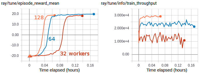
../_images/impala.png — Multi-GPU IMPALA scales up to solve PongNoFrameskip-v4 in ~3 minutes using a pair of V100 GPUs and 128 CPU workers. The maximum training throughput reached is ~30k transitions per second (~120k environment frames per second).#

IMPALA-specific configs (see also common configs):

class ray.rllib.algorithms.impala.impala.IMPALAConfig(algo_class=None)[source]#

Defines a configuration class from which an Impala can be built.

from ray.rllib.algorithms.impala import IMPALAConfig

config = (
    IMPALAConfig()
    .environment("CartPole-v1")
    .env_runners(num_env_runners=1)
    .training(lr=0.0003, train_batch_size_per_learner=512)
    .learners(num_learners=1)
)
# Build a Algorithm object from the config and run 1 training iteration.
algo = config.build()
algo.train()
del algo

from ray.rllib.algorithms.impala import IMPALAConfig
from ray import air
from ray import tune

config = (
    IMPALAConfig()
    .environment("CartPole-v1")
    .env_runners(num_env_runners=1)
    .training(lr=tune.grid_search([0.0001, 0.0002]), grad_clip=20.0)
    .learners(num_learners=1)
)
# Run with tune.
tune.Tuner(
    "IMPALA",
    param_space=config,
    run_config=air.RunConfig(stop={"training_iteration": 1}),
).fit()

training(*, vtrace: bool | None = <ray.rllib.utils.from_config._NotProvided object>, vtrace_clip_rho_threshold: float | None = <ray.rllib.utils.from_config._NotProvided object>, vtrace_clip_pg_rho_threshold: float | None = <ray.rllib.utils.from_config._NotProvided object>, gamma: float | None = <ray.rllib.utils.from_config._NotProvided object>, num_gpu_loader_threads: int | None = <ray.rllib.utils.from_config._NotProvided object>, num_multi_gpu_tower_stacks: int | None = <ray.rllib.utils.from_config._NotProvided object>, minibatch_buffer_size: int | None = <ray.rllib.utils.from_config._NotProvided object>, replay_proportion: float | None = <ray.rllib.utils.from_config._NotProvided object>, replay_buffer_num_slots: int | None = <ray.rllib.utils.from_config._NotProvided object>, learner_queue_size: int | None = <ray.rllib.utils.from_config._NotProvided object>, learner_queue_timeout: float | None = <ray.rllib.utils.from_config._NotProvided object>, max_requests_in_flight_per_aggregator_worker: int | None = <ray.rllib.utils.from_config._NotProvided object>, timeout_s_sampler_manager: float | None = <ray.rllib.utils.from_config._NotProvided object>, timeout_s_aggregator_manager: float | None = <ray.rllib.utils.from_config._NotProvided object>, broadcast_interval: int | None = <ray.rllib.utils.from_config._NotProvided object>, num_aggregation_workers: int | None = <ray.rllib.utils.from_config._NotProvided object>, grad_clip: float | None = <ray.rllib.utils.from_config._NotProvided object>, opt_type: str | None = <ray.rllib.utils.from_config._NotProvided object>, lr_schedule: ~typing.List[~typing.List[int | float]] | None = <ray.rllib.utils.from_config._NotProvided object>, decay: float | None = <ray.rllib.utils.from_config._NotProvided object>, momentum: float | None = <ray.rllib.utils.from_config._NotProvided object>, epsilon: float | None = <ray.rllib.utils.from_config._NotProvided object>, vf_loss_coeff: float | None = <ray.rllib.utils.from_config._NotProvided object>, entropy_coeff: float | ~typing.List[~typing.List[int | float]] | ~typing.List[~typing.Tuple[int, int | float]] | None = <ray.rllib.utils.from_config._NotProvided object>, entropy_coeff_schedule: ~typing.List[~typing.List[int | float]] | None = <ray.rllib.utils.from_config._NotProvided object>, _separate_vf_optimizer: bool | None = <ray.rllib.utils.from_config._NotProvided object>, _lr_vf: float | None = <ray.rllib.utils.from_config._NotProvided object>, after_train_step=-1, **kwargs) → IMPALAConfig[source]#

Sets the training related configuration.

Parameters:

vtrace – V-trace params (see vtrace_tf/torch.py).
vtrace_clip_rho_threshold
vtrace_clip_pg_rho_threshold
gamma – Float specifying the discount factor of the Markov Decision process.
num_gpu_loader_threads – The number of GPU-loader threads (per Learner worker), used to load incoming (CPU) batches to the GPU, if applicable. The incoming batches are produced by each Learner’s LearnerConnector pipeline. After loading the batches on the GPU, the threads place them on yet another queue for the Learner thread (only one per Learner worker) to pick up and perform forward_train/loss computations.
num_multi_gpu_tower_stacks – For each stack of multi-GPU towers, how many slots should we reserve for parallel data loading? Set this to >1 to load data into GPUs in parallel. This will increase GPU memory usage proportionally with the number of stacks. Example: 2 GPUs and num_multi_gpu_tower_stacks=3: - One tower stack consists of 2 GPUs, each with a copy of the model/graph. - Each of the stacks will create 3 slots for batch data on each of its GPUs, increasing memory requirements on each GPU by 3x. - This enables us to preload data into these stacks while another stack is performing gradient calculations.
minibatch_buffer_size – How many train batches should be retained for minibatching. This conf only has an effect if num_epochs > 1.
replay_proportion – Set >0 to enable experience replay. Saved samples will be replayed with a p:1 proportion to new data samples.
replay_buffer_num_slots – Number of sample batches to store for replay. The number of transitions saved total will be (replay_buffer_num_slots * rollout_fragment_length).
learner_queue_size – Max queue size for train batches feeding into the learner.
learner_queue_timeout – Wait for train batches to be available in minibatch buffer queue this many seconds. This may need to be increased e.g. when training with a slow environment.
max_requests_in_flight_per_aggregator_worker – Level of queuing for replay aggregator operations (if using aggregator workers).
timeout_s_sampler_manager – The timeout for waiting for sampling results for workers – typically if this is too low, the manager won’t be able to retrieve ready sampling results.
timeout_s_aggregator_manager – The timeout for waiting for replay worker results – typically if this is too low, the manager won’t be able to retrieve ready replay requests.
broadcast_interval – Number of training step calls before weights are broadcasted to rollout workers that are sampled during any iteration.
num_aggregation_workers – Use n (num_aggregation_workers) extra Actors for multi-level aggregation of the data produced by the m RolloutWorkers (num_env_runners). Note that n should be much smaller than m. This can make sense if ingesting >2GB/s of samples, or if the data requires decompression.
grad_clip – If specified, clip the global norm of gradients by this amount.
opt_type – Either “adam” or “rmsprop”.
lr_schedule – Learning rate schedule. In the format of [[timestep, lr-value], [timestep, lr-value], …] Intermediary timesteps will be assigned to interpolated learning rate values. A schedule should normally start from timestep 0.
decay – Decay setting for the RMSProp optimizer, in case opt_type=rmsprop.
momentum – Momentum setting for the RMSProp optimizer, in case opt_type=rmsprop.
epsilon – Epsilon setting for the RMSProp optimizer, in case opt_type=rmsprop.
vf_loss_coeff – Coefficient for the value function term in the loss function.
entropy_coeff – Coefficient for the entropy regularizer term in the loss function.
entropy_coeff_schedule – Decay schedule for the entropy regularizer.
_separate_vf_optimizer – Set this to true to have two separate optimizers optimize the policy-and value networks. Only supported for some algorithms (APPO, IMPALA) on the old API stack.
_lr_vf – If _separate_vf_optimizer is True, define separate learning rate for the value network.

Returns:

This updated AlgorithmConfig object.

Model-based RL#

DreamerV3#

[paper] [implementation]

Tuned examples: Atari 100k, Atari 200M, DeepMind Control Suite

Pong-v5 results (1, 2, and 4 GPUs):

../_images/pong_1_2_and_4gpus.svg — Episode mean rewards for the Pong-v5 environment (with the “100k” setting, in which only 100k environment steps are allowed): Note that despite the stable sample efficiency - shown by the constant learning performance per env step - the wall time improves almost linearly as we go from 1 to 4 GPUs. **Left**: Episode reward over environment timesteps sampled. **Right**: Episode reward over wall-time.#

Atari 100k results (1 vs 4 GPUs):

../_images/atari100k_1_vs_4gpus.svg — Episode mean rewards for various Atari 100k tasks on 1 vs 4 GPUs. **Left**: Episode reward over environment timesteps sampled. **Right**: Episode reward over wall-time.#

DeepMind Control Suite (vision) results (1 vs 4 GPUs):

../_images/dmc_1_vs_4gpus.svg — Episode mean rewards for various Atari 100k tasks on 1 vs 4 GPUs. **Left**: Episode reward over environment timesteps sampled. **Right**: Episode reward over wall-time.#

Offline RL and Imitation Learning#

Behavior Cloning (BC)#

[paper] [implementation]

../_images/bc-architecture.svg — **BC architecture:** RLlib’s behavioral cloning (BC) uses Ray Data to tap into its parallel data processing capabilities. In one training iteration, BC reads episodes in parallel from offline files, for example parquet, by the n DataWorkers. Connector pipelines then preprocess these episodes into train batches and send these as data iterators directly to the n Learners for updating the model. RLlib’s (BC) implementation is directly derived from its MARWIL implementation, with the only difference being the `beta` parameter (set to 0.0). This makes BC try to match the behavior policy, which generated the offline data, disregarding any resulting rewards.#

Tuned examples: CartPole-v1 Pendulum-v1

BC-specific configs (see also common configs):

class ray.rllib.algorithms.bc.bc.BCConfig(algo_class=None)[source]#

Defines a configuration class from which a new BC Algorithm can be built

from ray.rllib.algorithms.bc import BCConfig
# Run this from the ray directory root.
config = BCConfig().training(lr=0.00001, gamma=0.99)
config = config.offline_data(
    input_="./rllib/tests/data/cartpole/large.json")

# Build an Algorithm object from the config and run 1 training iteration.
algo = config.build()
algo.train()

from ray.rllib.algorithms.bc import BCConfig
from ray import tune
config = BCConfig()
# Print out some default values.
print(config.beta)
# Update the config object.
config.training(
    lr=tune.grid_search([0.001, 0.0001]), beta=0.75
)
# Set the config object's data path.
# Run this from the ray directory root.
config.offline_data(
    input_="./rllib/tests/data/cartpole/large.json"
)
# Set the config object's env, used for evaluation.
config.environment(env="CartPole-v1")
# Use to_dict() to get the old-style python config dict
# when running with tune.
tune.Tuner(
    "BC",
    param_space=config.to_dict(),
).fit()

training(*, beta: float | None = <ray.rllib.utils.from_config._NotProvided object>, bc_logstd_coeff: float | None = <ray.rllib.utils.from_config._NotProvided object>, moving_average_sqd_adv_norm_update_rate: float | None = <ray.rllib.utils.from_config._NotProvided object>, moving_average_sqd_adv_norm_start: float | None = <ray.rllib.utils.from_config._NotProvided object>, vf_coeff: float | None = <ray.rllib.utils.from_config._NotProvided object>, grad_clip: float | None = <ray.rllib.utils.from_config._NotProvided object>, **kwargs) → MARWILConfig#

Sets the training related configuration.

Parameters:

beta – Scaling of advantages in exponential terms. When beta is 0.0, MARWIL is reduced to behavior cloning (imitation learning); see bc.py algorithm in this same directory.
bc_logstd_coeff – A coefficient to encourage higher action distribution entropy for exploration.
moving_average_sqd_adv_norm_update_rate – The rate for updating the squared moving average advantage norm (c^2). A higher rate leads to faster updates of this moving avergage.
moving_average_sqd_adv_norm_start – Starting value for the squared moving average advantage norm (c^2).
vf_coeff – Balancing value estimation loss and policy optimization loss.
grad_clip – If specified, clip the global norm of gradients by this amount.

Returns:

This updated AlgorithmConfig object.

Conservative Q-Learning (CQL)#

[paper] [implementation]

../_images/cql-architecture.svg — **CQL architecture:** CQL (Conservative Q-Learning) is an offline RL algorithm that mitigates the overestimation of Q-values outside the dataset distribution through a conservative critic estimate. It adds a simple Q regularizer loss to the standard Bellman update loss, ensuring that the critic doesn’t output overly optimistic Q-values. The `SACLearner` adds this conservative correction term to the TD-based Q-learning loss.#

Tuned examples: Pendulum-v1

CQL-specific configs and common configs):

class ray.rllib.algorithms.cql.cql.CQLConfig(algo_class=None)[source]#

Defines a configuration class from which a CQL can be built.

from ray.rllib.algorithms.cql import CQLConfig
config = CQLConfig().training(gamma=0.9, lr=0.01)
config = config.resources(num_gpus=0)
config = config.env_runners(num_env_runners=4)
print(config.to_dict())
# Build a Algorithm object from the config and run 1 training iteration.
algo = config.build(env="CartPole-v1")
algo.train()

training(*, bc_iters: int | None = <ray.rllib.utils.from_config._NotProvided object>, temperature: float | None = <ray.rllib.utils.from_config._NotProvided object>, num_actions: int | None = <ray.rllib.utils.from_config._NotProvided object>, lagrangian: bool | None = <ray.rllib.utils.from_config._NotProvided object>, lagrangian_thresh: float | None = <ray.rllib.utils.from_config._NotProvided object>, min_q_weight: float | None = <ray.rllib.utils.from_config._NotProvided object>, deterministic_backup: bool | None = <ray.rllib.utils.from_config._NotProvided object>, **kwargs) → CQLConfig[source]#

Sets the training-related configuration.

Parameters:

bc_iters – Number of iterations with Behavior Cloning pretraining.
temperature – CQL loss temperature.
num_actions – Number of actions to sample for CQL loss
lagrangian – Whether to use the Lagrangian for Alpha Prime (in CQL loss).
lagrangian_thresh – Lagrangian threshold.
min_q_weight – in Q weight multiplier.
deterministic_backup – If the target in the Bellman update should have an entropy backup. Defaults to True.

Returns:

This updated AlgorithmConfig object.

Monotonic Advantage Re-Weighted Imitation Learning (MARWIL)#

[paper] [implementation]

../_images/marwil-architecture.svg — **MARWIL architecture:** MARWIL is a hybrid imitation learning and policy gradient algorithm suitable for training on batched historical data. When the `beta` hyperparameter is set to zero, the MARWIL objective reduces to plain imitation learning (see BC). MARWIL uses Ray.Data to tap into its parallel data processing capabilities. In one training iteration, MARWIL reads episodes in parallel from offline files, for example parquet, by the n DataWorkers. Connector pipelines preprocess these episodes into train batches and send these as data iterators directly to the n Learners for updating the model.#

Tuned examples: CartPole-v1

MARWIL-specific configs (see also common configs):

class ray.rllib.algorithms.marwil.marwil.MARWILConfig(algo_class=None)[source]#

Defines a configuration class from which a MARWIL Algorithm can be built.

import gymnasium as gym
import numpy as np

from pathlib import Path
from ray.rllib.algorithms.marwil import MARWILConfig

# Get the base path (to ray/rllib)
base_path = Path(__file__).parents[2]
# Get the path to the data in rllib folder.
data_path = base_path / "tests/data/cartpole/cartpole-v1_large"

config = MARWILConfig()
# Enable the new API stack.
config.api_stack(
    enable_rl_module_and_learner=True,
    enable_env_runner_and_connector_v2=True,
)
# Define the environment for which to learn a policy
# from offline data.
config.environment(
    observation_space=gym.spaces.Box(
        np.array([-4.8, -np.inf, -0.41887903, -np.inf]),
        np.array([4.8, np.inf, 0.41887903, np.inf]),
        shape=(4,),
        dtype=np.float32,
    ),
    action_space=gym.spaces.Discrete(2),
)
# Set the training parameters.
config.training(
    beta=1.0,
    lr=1e-5,
    gamma=0.99,
    # We must define a train batch size for each
    # learner (here 1 local learner).
    train_batch_size_per_learner=2000,
)
# Define the data source for offline data.
config.offline_data(
    input_=[data_path.as_posix()],
    # Run exactly one update per training iteration.
    dataset_num_iters_per_learner=1,
)

# Build an `Algorithm` object from the config and run 1 training
# iteration.
algo = config.build()
algo.train()

import gymnasium as gym
import numpy as np

from pathlib import Path
from ray.rllib.algorithms.marwil import MARWILConfig
from ray import train, tune

# Get the base path (to ray/rllib)
base_path = Path(__file__).parents[2]
# Get the path to the data in rllib folder.
data_path = base_path / "tests/data/cartpole/cartpole-v1_large"

config = MARWILConfig()
# Enable the new API stack.
config.api_stack(
    enable_rl_module_and_learner=True,
    enable_env_runner_and_connector_v2=True,
)
# Print out some default values
print(f"beta: {config.beta}")
# Update the config object.
config.training(
    lr=tune.grid_search([1e-3, 1e-4]),
    beta=0.75,
    # We must define a train batch size for each
    # learner (here 1 local learner).
    train_batch_size_per_learner=2000,
)
# Set the config's data path.
config.offline_data(
    input_=[data_path.as_posix()],
    # Set the number of updates to be run per learner
    # per training step.
    dataset_num_iters_per_learner=1,
)
# Set the config's environment for evalaution.
config.environment(
    observation_space=gym.spaces.Box(
        np.array([-4.8, -np.inf, -0.41887903, -np.inf]),
        np.array([4.8, np.inf, 0.41887903, np.inf]),
        shape=(4,),
        dtype=np.float32,
    ),
    action_space=gym.spaces.Discrete(2),
)
# Set up a tuner to run the experiment.
tuner = tune.Tuner(
    "MARWIL",
    param_space=config,
    run_config=train.RunConfig(
        stop={"training_iteration": 1},
    ),
)
# Run the experiment.
tuner.fit()

Sets the training related configuration.

Parameters:

beta – Scaling of advantages in exponential terms. When beta is 0.0, MARWIL is reduced to behavior cloning (imitation learning); see bc.py algorithm in this same directory.
bc_logstd_coeff – A coefficient to encourage higher action distribution entropy for exploration.
moving_average_sqd_adv_norm_update_rate – The rate for updating the squared moving average advantage norm (c^2). A higher rate leads to faster updates of this moving avergage.
moving_average_sqd_adv_norm_start – Starting value for the squared moving average advantage norm (c^2).
vf_coeff – Balancing value estimation loss and policy optimization loss.
grad_clip – If specified, clip the global norm of gradients by this amount.

Returns:

This updated AlgorithmConfig object.

Algorithm Extensions- and Plugins#

Curiosity-driven Exploration by Self-supervised Prediction#

[paper] [implementation]

../_images/curiosity-architecture.svg — **Intrinsic Curiosity Model (ICM) architecture:** The main idea behind ICM is to train a world-model (in parallel to the “main” policy) to predict the environment’s dynamics. The loss of the world model is the intrinsic reward that the `ICMLearner` adds to the env’s (extrinsic) reward. This makes sure that when in regions of the environment that are relatively unknown (world model performs badly in predicting what happens next), the artificial intrinsic reward is large and the agent is motivated to go and explore these unknown regions. RLlib’s curiosity implementation works with any of RLlib’s algorithms. See these links here for example implementations on top of PPO and DQN. ICM uses the chosen Algorithm’s `training_step()` as-is, but then executes the following additional steps during `LearnerGroup.update`: Duplicate the train batch of the “main” policy and use it for performing a self-supervised update of the ICM. Use the ICM to compute the intrinsic rewards and add these to the extrinsic (env) rewards. Then continue updating the “main” policy.#

Tuned examples: 12x12 FrozenLake-v1