Distributed training

 

 

This tutorial executes a distributed training workload that connects the following heterogeneous workloads:

• preprocess the dataset prior to training

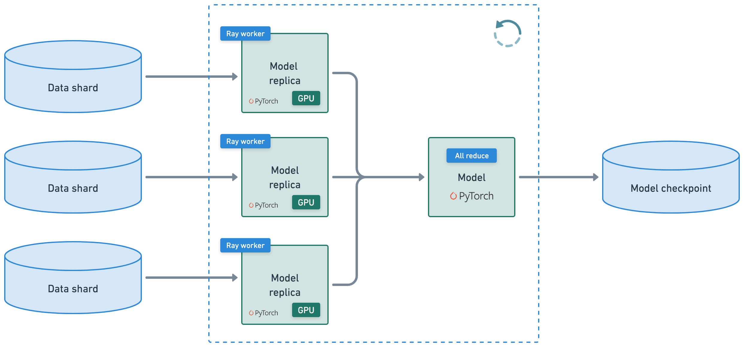
• distributed training with Ray Train and PyTorch with observability

• evaluation (batch inference and eval logic)

• save model artifacts to a model registry (MLOps)

Note: this tutorial doesn’t tune the model but see Ray Tune for experiment execution and hyperparameter tuning at any scale.

%%bash
pip install -q -r /home/ray/default/requirements.txt
pip install -q -e /home/ray/default/doggos

Note: A kernel restart may be required for all dependencies to become available.

If using uv, then:

1. Turn off the runtime dependencies (Dependencies tab up top > Toggle off Pip packages). And no need to run the pip install commands above.

2. Change the python kernel of this notebook to use the venv (Click on base (Python x.yy.zz) on top right cordern of notebook > Select another Kernel > Python Environments... > Create Python Environment > Venv > Use Existing) and done! Now all the notebook’s cells will use the virtual env.

3. Change the py executable to use uv run instead of python by adding this line after importing ray.

import os
os.environ.pop("RAY_RUNTIME_ENV_HOOK", None)
import ray
ray.init(runtime_env={"py_executable": "uv run", "working_dir": "/home/ray/default"})

%load_ext autoreload
%autoreload all

import os
import ray
import sys
sys.path.append(os.path.abspath("../doggos/"))

# If using UV
# os.environ.pop("RAY_RUNTIME_ENV_HOOK", None)

# Enable Ray Train v2. It's too good to wait for public release!
os.environ["RAY_TRAIN_V2_ENABLED"] = "1"
ray.init(
    # connect to existing ray runtime (from previous notebook if still running)
    address=os.environ.get("RAY_ADDRESS", "auto"),
    runtime_env={
        "env_vars": {"RAY_TRAIN_V2_ENABLED": "1"},
        # "py_executable": "uv run", # if using uv 
        # "working_dir": "/home/ray/default",  # if using uv 
    },
)

%%bash
# This will be removed once Ray Train v2 is enabled by default.
echo "RAY_TRAIN_V2_ENABLED=1" > /home/ray/default/.env

# Load env vars in notebooks.
from dotenv import load_dotenv
load_dotenv()

Preprocess

You need to convert the classes to labels (unique integers) so that you can train a classifier that can correctly predict the class given an input image. But before you do this, apply the same data ingestion and preprocessing as the previous notebook.

def add_class(row):
    row["class"] = row["path"].rsplit("/", 3)[-2]
    return row

# Preprocess data splits.
train_ds = ray.data.read_images("s3://doggos-dataset/train", include_paths=True, shuffle="files")
train_ds = train_ds.map(add_class)
val_ds = ray.data.read_images("s3://doggos-dataset/val", include_paths=True)
val_ds = val_ds.map(add_class)

Define a Preprocessor class that:

• creates an embedding. A later step moves the embedding layer outside of the model since you freeze the embedding layer’s weights and so you don’t have to do it repeatedly as part of the model’s forward pass, saving on unnecessary compute.

• convert the classes into labels for the classifier.

While you could’ve just done this step as a simple operation, you’re taking the time to organize it as a class so that you can save and load for inference later.

def convert_to_label(row, class_to_label):
    if "class" in row:
        row["label"] = class_to_label[row["class"]]
    return row

import numpy as np
from PIL import Image
import torch
from transformers import CLIPModel, CLIPProcessor
from doggos.embed import EmbedImages

class Preprocessor:
    """Preprocessor class."""
    def __init__(self, class_to_label=None):
        self.class_to_label = class_to_label or {}  # mutable defaults
        self.label_to_class = {v: k for k, v in self.class_to_label.items()}
        
    def fit(self, ds, column):
        self.classes = ds.unique(column=column)
        self.class_to_label = {tag: i for i, tag in enumerate(self.classes)}
        self.label_to_class = {v: k for k, v in self.class_to_label.items()}
        return self
    
    def transform(self, ds, concurrency=4, batch_size=64, num_gpus=1):
        ds = ds.map(
            convert_to_label, 
            fn_kwargs={"class_to_label": self.class_to_label},
        )
        ds = ds.map_batches(
            EmbedImages,
            fn_constructor_kwargs={
                "model_id": "openai/clip-vit-base-patch32", 
                "device": "cuda",
            },
            concurrency=4,
            batch_size=64,
            num_gpus=1,
            accelerator_type="T4",
        )
        ds = ds.drop_columns(["image"])
        return ds

    def save(self, fp):
        with open(fp, "w") as f:
            json.dump(self.class_to_label, f)

# Preprocess.
preprocessor = Preprocessor()
preprocessor = preprocessor.fit(train_ds, column="class")
train_ds = preprocessor.transform(ds=train_ds)
val_ds = preprocessor.transform(ds=val_ds)

Data processing

See this extensive guide on data loading and preprocessing for the last-mile preprocessing you need to do prior to training your models. However, Ray Data does support performant joins, filters, aggregations, etc., for the more structure data processing your workloads may need.

import shutil

# Write processed data to cloud storage.
preprocessed_data_path = os.path.join("/mnt/cluster_storage", "doggos/preprocessed_data")
if os.path.exists(preprocessed_data_path):  # Clean up.
    shutil.rmtree(preprocessed_data_path)
preprocessed_train_path = os.path.join(preprocessed_data_path, "preprocessed_train")
preprocessed_val_path = os.path.join(preprocessed_data_path, "preprocessed_val")
train_ds.write_parquet(preprocessed_train_path)
val_ds.write_parquet(preprocessed_val_path)

Store often, save compute

Store the preprocessed data into shared cloud storage to:

• save a record of what this preprocessed data looks like

• avoid triggering the entire preprocessing for each batch the model processes

• avoid materialize of the preprocessed data because you shouldn’t force large data to fit in memory

Model

Define the model – a simple two layer neural net with Softmax layer to predict class probabilities. Notice that it’s all just base PyTorch and nothing else.

import json
from pathlib import Path
import torch
import torch.nn as nn
import torch.nn.functional as F

class ClassificationModel(torch.nn.Module):
    def __init__(self, embedding_dim, hidden_dim, dropout_p, num_classes):
        super().__init__()
        # Hyperparameters
        self.embedding_dim = embedding_dim
        self.hidden_dim = hidden_dim
        self.dropout_p = dropout_p
        self.num_classes = num_classes

        # Define layers
        self.fc1 = nn.Linear(embedding_dim, hidden_dim)
        self.batch_norm = nn.BatchNorm1d(hidden_dim)
        self.relu = nn.ReLU()
        self.dropout = nn.Dropout(dropout_p)
        self.fc2 = nn.Linear(hidden_dim, num_classes)

    def forward(self, batch):
        z = self.fc1(batch["embedding"])
        z = self.batch_norm(z)
        z = self.relu(z)
        z = self.dropout(z)
        z = self.fc2(z)
        return z

    @torch.inference_mode()
    def predict(self, batch):
        z = self(batch)
        y_pred = torch.argmax(z, dim=1).cpu().numpy()
        return y_pred

    @torch.inference_mode()
    def predict_probabilities(self, batch):
        z = self(batch)
        y_probs = F.softmax(z, dim=1).cpu().numpy()
        return y_probs

    def save(self, dp):
        Path(dp).mkdir(parents=True, exist_ok=True)
        with open(Path(dp, "args.json"), "w") as fp:
            json.dump({
                "embedding_dim": self.embedding_dim,
                "hidden_dim": self.hidden_dim,
                "dropout_p": self.dropout_p,
                "num_classes": self.num_classes,
            }, fp, indent=4)
        torch.save(self.state_dict(), Path(dp, "model.pt"))

    @classmethod
    def load(cls, args_fp, state_dict_fp, device="cpu"):
        with open(args_fp, "r") as fp:
            model = cls(**json.load(fp))
        model.load_state_dict(torch.load(state_dict_fp, map_location=device))
        return model

# Initialize model.
num_classes = len(preprocessor.classes)
model = ClassificationModel(
    embedding_dim=512, 
    hidden_dim=256, 
    dropout_p=0.3, 
    num_classes=num_classes,
)
print (model)

Batching

Take a look at a sample batch of data and ensure that tensors have the proper data type.

from ray.train.torch import get_device

def collate_fn(batch, device=None):
    dtypes = {"embedding": torch.float32, "label": torch.int64}
    tensor_batch = {}
    
    # If no device is provided, try to get it from Ray Train context
    if device is None:
        try:
            device = get_device()
        except RuntimeError:
            # When not in Ray Train context, use CPU for testing
            device = "cpu"
    
    for key in dtypes.keys():
        if key in batch:
            tensor_batch[key] = torch.as_tensor(
                batch[key],
                dtype=dtypes[key],
                device=device,
            )
    return tensor_batch

# Sample batch
sample_batch = train_ds.take_batch(batch_size=3)
collate_fn(batch=sample_batch, device="cpu")

Model registry

Create a model registry in Anyscale user storage to save the model checkpoints to. Use OSS MLflow but you can easily set up other experiment trackers with Ray.

import shutil

model_registry = "/mnt/cluster_storage/mlflow/doggos"
if os.path.isdir(model_registry):
    shutil.rmtree(model_registry)  # clean up
os.makedirs(model_registry, exist_ok=True)

Training

Define the training workload by specifying the:

• experiment and model parameters

• compute scaling configuration

• forward pass for batches of training and validation data

• train loop for each epoch of data and checkpointing

# Train loop config.
experiment_name = "doggos"
train_loop_config = {
    "model_registry": model_registry,
    "experiment_name": experiment_name,
    "embedding_dim": 512,
    "hidden_dim": 256,
    "dropout_p": 0.3,
    "lr": 1e-3,
    "lr_factor": 0.8,
    "lr_patience": 3,
    "num_epochs": 20,
    "batch_size": 256,
}

# Scaling config
num_workers = 4
scaling_config = ray.train.ScalingConfig(
    num_workers=num_workers,
    use_gpu=True,
    resources_per_worker={"CPU": 8, "GPU": 2},
    accelerator_type="T4",
)

import tempfile
import mlflow
import numpy as np
from ray.train.torch import TorchTrainer

def train_epoch(ds, batch_size, model, num_classes, loss_fn, optimizer):
    model.train()
    loss = 0.0
    ds_generator = ds.iter_torch_batches(batch_size=batch_size, collate_fn=collate_fn)
    for i, batch in enumerate(ds_generator):
        optimizer.zero_grad()  # Reset gradients.
        z = model(batch)  # Forward pass.
        targets = F.one_hot(batch["label"], num_classes=num_classes).float()
        J = loss_fn(z, targets)  # Define loss.
        J.backward()  # Backward pass.
        optimizer.step()  # Update weights.
        loss += (J.detach().item() - loss) / (i + 1)  # Cumulative loss
    return loss

def eval_epoch(ds, batch_size, model, num_classes, loss_fn):
    model.eval()
    loss = 0.0
    y_trues, y_preds = [], []
    ds_generator = ds.iter_torch_batches(batch_size=batch_size, collate_fn=collate_fn)
    with torch.inference_mode():
        for i, batch in enumerate(ds_generator):
            z = model(batch)
            targets = F.one_hot(batch["label"], num_classes=num_classes).float()  # one-hot (for loss_fn)
            J = loss_fn(z, targets).item()
            loss += (J - loss) / (i + 1)
            y_trues.extend(batch["label"].cpu().numpy())
            y_preds.extend(torch.argmax(z, dim=1).cpu().numpy())
    return loss, np.vstack(y_trues), np.vstack(y_preds)

def train_loop_per_worker(config):
    # Hyperparameters.
    model_registry = config["model_registry"]
    experiment_name = config["experiment_name"]
    embedding_dim = config["embedding_dim"]
    hidden_dim = config["hidden_dim"]
    dropout_p = config["dropout_p"]
    lr = config["lr"]
    lr_factor = config["lr_factor"]
    lr_patience = config["lr_patience"]
    num_epochs = config["num_epochs"]
    batch_size = config["batch_size"]
    num_classes = config["num_classes"]

    # Experiment tracking.
    if ray.train.get_context().get_world_rank() == 0:
        mlflow.set_tracking_uri(f"file:{model_registry}")
        mlflow.set_experiment(experiment_name)
        mlflow.start_run()
        mlflow.log_params(config)

    # Datasets.
    train_ds = ray.train.get_dataset_shard("train")
    val_ds = ray.train.get_dataset_shard("val")

    # Model.
    model = ClassificationModel(
        embedding_dim=embedding_dim, 
        hidden_dim=hidden_dim, 
        dropout_p=dropout_p, 
        num_classes=num_classes,
    )
    model = ray.train.torch.prepare_model(model)

    # Training components.
    loss_fn = torch.nn.CrossEntropyLoss()
    optimizer = torch.optim.Adam(model.parameters(), lr=lr)
    scheduler = torch.optim.lr_scheduler.ReduceLROnPlateau(
        optimizer, 
        mode="min", 
        factor=lr_factor, 
        patience=lr_patience,
    )

    # Training.
    best_val_loss = float("inf")
    for epoch in range(num_epochs):
        # Steps
        train_loss = train_epoch(train_ds, batch_size, model, num_classes, loss_fn, optimizer)
        val_loss, _, _ = eval_epoch(val_ds, batch_size, model, num_classes, loss_fn)
        scheduler.step(val_loss)

        # Checkpoint (metrics, preprocessor and model artifacts).
        with tempfile.TemporaryDirectory() as dp:
            model.module.save(dp=dp)
            metrics = dict(lr=optimizer.param_groups[0]["lr"], train_loss=train_loss, val_loss=val_loss)
            with open(os.path.join(dp, "class_to_label.json"), "w") as fp:
                json.dump(config["class_to_label"], fp, indent=4)
            if ray.train.get_context().get_world_rank() == 0:  # only on main worker 0
                mlflow.log_metrics(metrics, step=epoch)
                if val_loss < best_val_loss:
                    best_val_loss = val_loss
                    mlflow.log_artifacts(dp)

    # End experiment tracking.
    if ray.train.get_context().get_world_rank() == 0:
        mlflow.end_run()

Minimal change to your training code

Notice that there isn’t much new Ray Train code on top of the base PyTorch code. You specified how you want to scale out the training workload, load the Ray datasets, and then checkpoint on the main worker node and that’s it. See these guides (PyTorch, PyTorch Lightning, Hugging Face Transformers) to see the minimal change in code needed to distribute your training workloads. See this extensive list of Ray Train user guides.

# Load preprocessed datasets.
preprocessed_train_ds = ray.data.read_parquet(preprocessed_train_path)
preprocessed_val_ds = ray.data.read_parquet(preprocessed_val_path)

# Trainer.
train_loop_config["class_to_label"] = preprocessor.class_to_label
train_loop_config["num_classes"] = len(preprocessor.class_to_label)
trainer = TorchTrainer(
    train_loop_per_worker=train_loop_per_worker,
    train_loop_config=train_loop_config,
    scaling_config=scaling_config,
    datasets={"train": preprocessed_train_ds, "val": preprocessed_val_ds},
)

# Train.
results = trainer.fit()

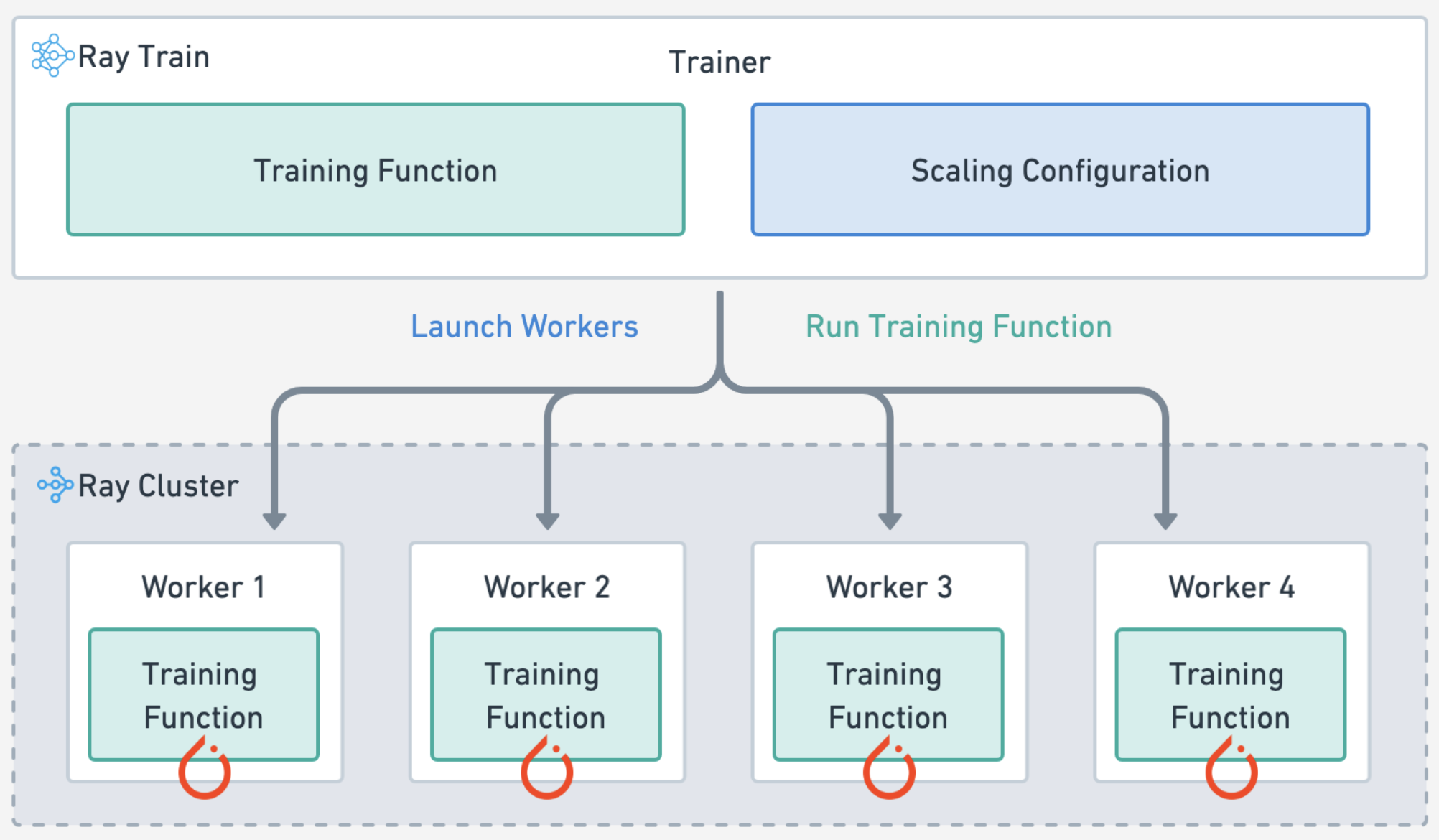
Ray Train

• automatically handles multi-node, multi-GPU setup with no manual SSH setup or hostfile configs.

• define per-worker fractional resource requirements, for example, 2 CPUs and 0.5 GPU per worker.

• run on heterogeneous machines and scale flexibly, for example, CPU for preprocessing and GPU for training.

• built-in fault tolerance with retry of failed workers and continue from last checkpoint.

• supports Data Parallel, Model Parallel, Parameter Server, and even custom strategies.

• Ray Compiled graphs allow you to even define different parallelism for jointly optimizing multiple models like Megatron, DeepSpeed, etc., or only allow for one global setting.

• You can also use Torch DDP, FSPD, DeepSpeed, etc., under the hood.

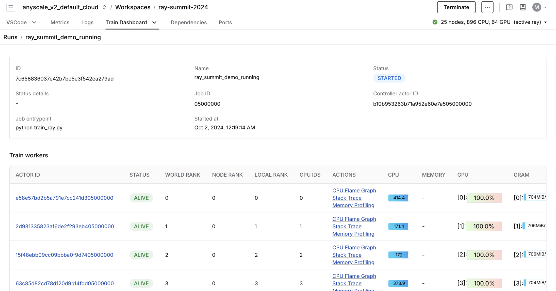
🔥 RayTurbo Train offers even more improvement to the price-performance ratio, performance monitoring and more:

• elastic training to scale to a dynamic number of workers, continue training on fewer resources, even on spot instances.

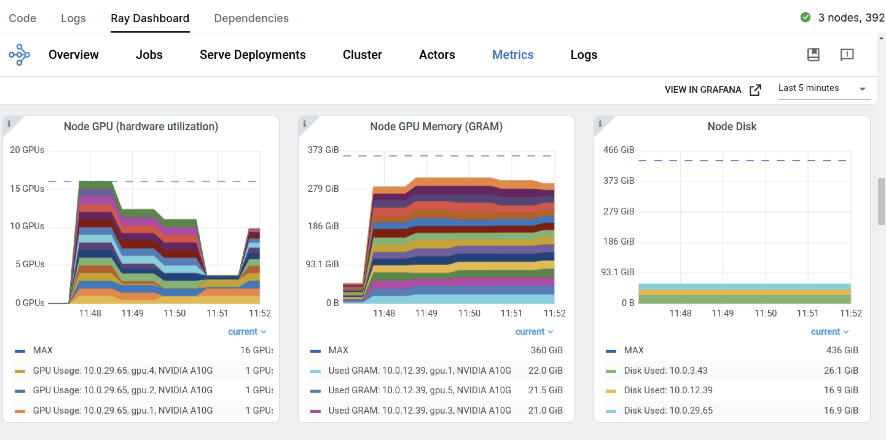
• purpose-built dashboard designed to streamline the debugging of Ray Train workloads:

  • Monitoring: View the status of training runs and train workers.

  • Metrics: See insights on training throughput and training system operation time.

  • Profiling: Investigate bottlenecks, hangs, or errors from individual training worker processes.

You can view experiment metrics and model artifacts in the model registry. You’re using OSS MLflow so you can run the server by pointing to the model registry location:

mlflow server -h 0.0.0.0 -p 8080 --backend-store-uri /mnt/cluster_storage/mlflow/doggos

You can view the dashboard by going to the Overview tab > Open Ports.

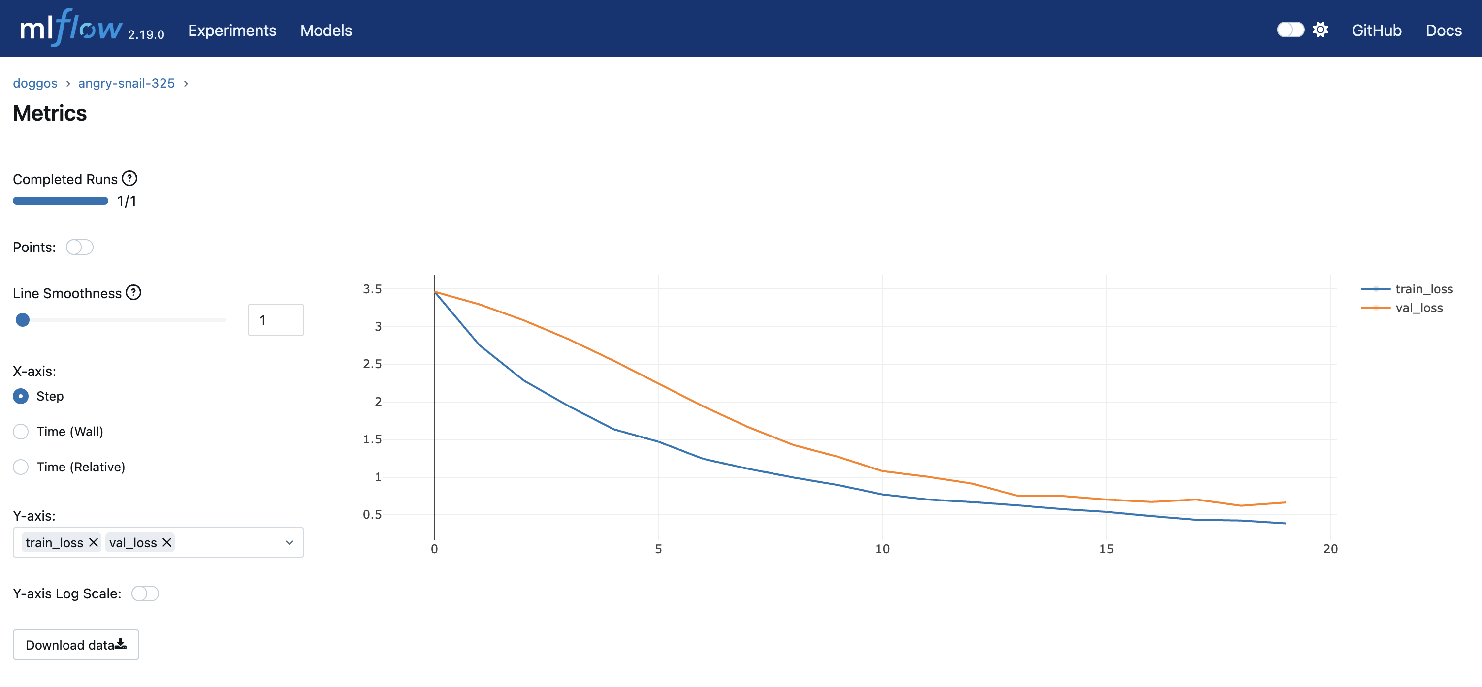
You also have the preceding Ray Dashboard and Train workload specific dashboards.

# Sorted runs
mlflow.set_tracking_uri(f"file:{model_registry}")
sorted_runs = mlflow.search_runs(
    experiment_names=[experiment_name], 
    order_by=["metrics.val_loss ASC"])
best_run = sorted_runs.iloc[0]
best_run

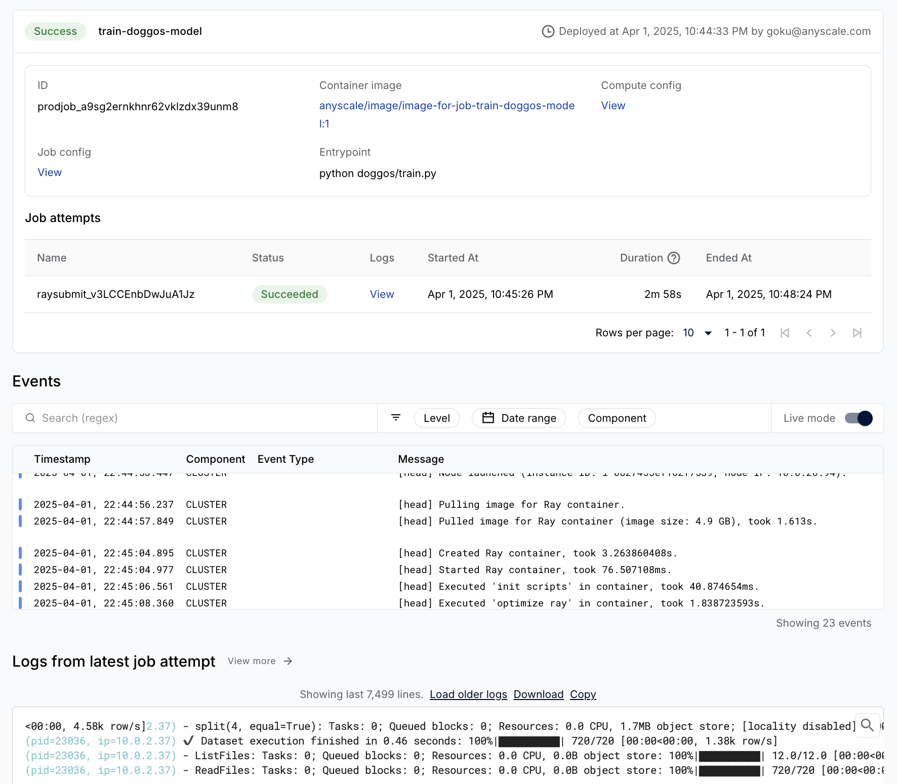
Production Job

You can easily wrap the training workload as a production grade Anyscale Job (API ref).

Note:

• This Job uses a containerfile to define dependencies, but you could easily use a pre-built image as well.

• You can specify the compute as a compute config or inline in a job config file.

• When you don’t specify compute while launching from a workspace, this configuration defaults to the compute configuration of the workspace.

%%bash
# Production model training job
anyscale job submit -f /home/ray/default/configs/train_model.yaml

Evaluation

This tutorial concludes by evaluating the trained model on the test dataset. Evaluation is essentially the same as the batch inference workload where you apply the model on batches of data and then calculate metrics using the predictions versus true labels. Ray Data is hyper optimized for throughput so preserving order isn’t a priority. But for evaluation, this approach is crucial. Achieve this approach by preserving the entire row and adding the predicted label as another column to each row.

from urllib.parse import urlparse
from sklearn.metrics import multilabel_confusion_matrix

class TorchPredictor:
    def __init__(self, preprocessor, model):
        self.preprocessor = preprocessor
        self.model = model
        self.model.eval()

    def __call__(self, batch, device="cuda"):
        self.model.to(device)
        batch["prediction"] = self.model.predict(collate_fn(batch, device=device))
        return batch

    def predict_probabilities(self, batch, device="cuda"):
        self.model.to(device)
        predicted_probabilities = self.model.predict_probabilities(collate_fn(batch, device=device))
        batch["probabilities"] = [
            {
                self.preprocessor.label_to_class[i]: float(prob)
                for i, prob in enumerate(probabilities)
            }
            for probabilities in predicted_probabilities
        ]
        return batch
    
    @classmethod
    def from_artifacts_dir(cls, artifacts_dir):
        with open(os.path.join(artifacts_dir, "class_to_label.json"), "r") as fp:
            class_to_label = json.load(fp)
        preprocessor = Preprocessor(class_to_label=class_to_label)
        model = ClassificationModel.load(
            args_fp=os.path.join(artifacts_dir, "args.json"), 
            state_dict_fp=os.path.join(artifacts_dir, "model.pt"),
        )
        return cls(preprocessor=preprocessor, model=model)

# Load and preproces eval dataset.
artifacts_dir = urlparse(best_run.artifact_uri).path
predictor = TorchPredictor.from_artifacts_dir(artifacts_dir=artifacts_dir)
test_ds = ray.data.read_images("s3://doggos-dataset/test", include_paths=True)
test_ds = test_ds.map(add_class)
test_ds = predictor.preprocessor.transform(ds=test_ds)

# y_pred (batch inference).
pred_ds = test_ds.map_batches(
    predictor,
    concurrency=4,
    batch_size=64,
    num_gpus=1,
    accelerator_type="T4",
)
pred_ds.take(1)

def batch_metric(batch):
    labels = batch["label"]
    preds = batch["prediction"]
    mcm = multilabel_confusion_matrix(labels, preds)
    tn, fp, fn, tp = [], [], [], []
    for i in range(mcm.shape[0]):
        tn.append(mcm[i, 0, 0])  # True negatives
        fp.append(mcm[i, 0, 1])  # False positives
        fn.append(mcm[i, 1, 0])  # False negatives
        tp.append(mcm[i, 1, 1])  # True positives
    return {"TN": tn, "FP": fp, "FN": fn, "TP": tp}

# Aggregated metrics after processing all batches.
metrics_ds = pred_ds.map_batches(batch_metric)
aggregate_metrics = metrics_ds.sum(["TN", "FP", "FN", "TP"])

# Aggregate the confusion matrix components across all batches.
tn = aggregate_metrics["sum(TN)"]
fp = aggregate_metrics["sum(FP)"]
fn = aggregate_metrics["sum(FN)"]
tp = aggregate_metrics["sum(TP)"]

# Calculate metrics.
precision = tp / (tp + fp) if (tp + fp) > 0 else 0
recall = tp / (tp + fn) if (tp + fn) > 0 else 0
f1 = 2 * precision * recall / (precision + recall) if (precision + recall) > 0 else 0
accuracy = (tp + tn) / (tp + tn + fp + fn)

print(f"Precision: {precision:.2f}")
print(f"Recall: {recall:.2f}")
print(f"F1: {f1:.2f}")
print(f"Accuracy: {accuracy:.2f}")

🚨 Note: Reset this notebook using the “🔄 Restart” button location at the notebook’s menu bar. This way we can free up all the variables, utils, etc. used in this notebook.