Working with offline data#
With RLlib’s offline RL API, you work with experiences read from offline storage such as disk, cloud storage, streaming systems, and the Hadoop Distributed File System (HDFS). You might read experiences saved from previous training runs, collected from experts, or gathered from policies deployed in web applications. You can also log new agent experiences produced during online training for later use.
RLlib represents trajectory sequences, such as (s, a, r, s', ...) tuples, with SingleAgentEpisode objects. RLlib doesn’t support multi-agent offline training. This episode format encodes and compresses experiences efficiently, rewrites trajectories, and gives you data access through getter methods. During online training, RLlib uses SingleAgentEnvRunner actors to generate episodes of experiences in parallel with the active policy. RLlib uses this same episode format to read experiences from and write experiences to offline storage. See OfflineSingleAgentEnvRunner.
You can store experiences directly in RLlib’s episode format or in a columnar table format. Use the episode format when either of the following applies:
You need experiences grouped by trajectory and ordered in time, such as to train stateful modules.
You want to use recorded experiences exclusively within RLlib, such as for offline RL or behavior cloning.
Prefer the columnar table format when you need to read the data with other data tools or ML libraries.
Note
RLlib’s new API stack incorporates principles that support standalone applications, so you can use the SingleAgentEpisode class outside an RLlib context. For faster access through external data tools, such as for data transformations, use the columnar table record format.
RLlib’s offline RL API builds on Ray Data, so it supports all of Ray Data’s read and write methods, such as read_parquet and read_json. The defaults are read_parquet for reading and write_parquet for writing. The API applies as many data transformations as possible on the fly before the data reaches the learner, so the learner focuses on model updates.
Hint
During the transition from the old API stack to the new one, you can use the offline RL API with SampleBatch data recorded on the old API stack. To enable this, set config.offline_data(input_read_sample_batches=True).
Example: Training an expert policy#
In this example you train a PPO agent on the CartPole-v1 environment until it reaches an episode mean return of 450.0. You checkpoint this agent and then use its policy to record expert data to local disk.
from ray.rllib.algorithms.ppo import PPOConfig
from ray.rllib.core.rl_module.default_model_config import DefaultModelConfig
from ray.rllib.utils.metrics import (
    ENV_RUNNER_RESULTS,
    EVALUATION_RESULTS,
    EPISODE_RETURN_MEAN,
)
from ray import tune

# Configure the PPO algorithm.
config = (
    PPOConfig()
    .environment("CartPole-v1")
    .training(
        lr=0.0003,
        # Run 6 SGD minibatch iterations on a batch.
        num_epochs=6,
        # Weigh the value function loss smaller than
        # the policy loss.
        vf_loss_coeff=0.01,
    )
    .rl_module(
        model_config=DefaultModelConfig(
            fcnet_hiddens=[32],
            fcnet_activation="linear",
            # Share encoder layers between value network
            # and policy.
            vf_share_layers=True,
        ),
    )
)

# Define the metric to use for stopping.
metric = f"{EVALUATION_RESULTS}/{ENV_RUNNER_RESULTS}/{EPISODE_RETURN_MEAN}"

# Define the Tuner.
tuner = tune.Tuner(
    "PPO",
    param_space=config,
    run_config=tune.RunConfig(
        stop={
            metric: 450.0,
        },
        name="docs_rllib_offline_pretrain_ppo",
        verbose=2,
        checkpoint_config=tune.CheckpointConfig(
            checkpoint_frequency=1,
            checkpoint_at_end=True,
        ),
    ),
)
results = tuner.fit()

# Store the best checkpoint to use it later for recording
# an expert policy.
best_checkpoint = (
    results
    .get_best_result(
        metric=metric,
        mode="max"
    )
    .checkpoint.path
)
In this example, you saved a checkpoint from an agent that has become an expert at playing CartPole-v1. You use this checkpoint in the next example to record expert data to disk, then use that data in offline training to clone another agent.
Example: Record expert data to local disk#
After you train an expert policy to play CartPole-v1, you load its policy to record expert data during evaluation. You use 5 OfflineSingleAgentEnvRunner instances to collect 50 complete episodes per sample() call. You store experiences directly in RLlib’s SingleAgentEpisode objects, with no more than 25 episode objects per Parquet file. You run 10 evaluation runs, which should produce 500 recorded episodes from the expert policy. You use this data in the next example to train a new policy through offline RL that should reach a return of 450.0 when playing CartPole-v1.
from ray.rllib.algorithms.ppo import PPOConfig
from ray.rllib.core import (
    COMPONENT_LEARNER_GROUP,
    COMPONENT_LEARNER,
    COMPONENT_RL_MODULE,
    DEFAULT_MODULE_ID,
)
from ray.rllib.core.rl_module import RLModuleSpec

# Store recording data under the following path.
data_path = "/tmp/docs_rllib_offline_recording"

# Configure the algorithm for recording.
config = (
    PPOConfig()
    # The environment needs to be specified.
    .environment(
        env="CartPole-v1",
    )
    # Make sure to sample complete episodes because
    # you want to record RLlib's episode objects.
    .env_runners(
        batch_mode="complete_episodes",
    )
    # Set up 5 evaluation `EnvRunners` for recording.
    # Sample 50 episodes in each evaluation rollout.
    .evaluation(
        evaluation_num_env_runners=5,
        evaluation_duration=50,
        evaluation_duration_unit="episodes",
    )
    # Use the checkpointed expert policy from the preceding PPO training.
    # Note, we have to use the same `model_config` as
    # the one with which the expert policy was trained, otherwise
    # the module state can't be loaded.
    .rl_module(
        model_config=DefaultModelConfig(
            fcnet_hiddens=[32],
            fcnet_activation="linear",
            # Share encoder layers between value network
            # and policy.
            vf_share_layers=True,
        ),
    )
    # Define the output path and format. In this example you
    # want to store data directly in RLlib's episode objects.
    # Each Parquet file should hold no more than 25 episodes.
    .offline_data(
        output=data_path,
        output_write_episodes=True,
        output_max_rows_per_file=25,
    )
)

# Build the algorithm.
algo = config.build()
# Load now the PPO-trained `RLModule` to use in recording.
algo.restore_from_path(
    best_checkpoint,
    # Load only the `RLModule` component here.
    component=COMPONENT_RL_MODULE,
)

# Run 10 evaluation iterations and record the data.
for i in range(10):
    print(f"Iteration {i + 1}")
    eval_results = algo.evaluate()
    print(eval_results)

# Stop the algorithm. Note, this is important for when
# defining `output_max_rows_per_file`. Otherwise,
# remaining episodes in the `EnvRunner`s buffer isn't written to disk.
algo.stop()
Note
RLlib formats the stored episode data as binary. It converts each episode into its dictionary representation and serializes it with msgpack-numpy, which ensures version compatibility.
RLlib’s recording process is efficient because it uses multiple OfflineSingleAgentEnvRunner instances during evaluation to write data in parallel. Explore the folder to review the stored Parquet data:
$ ls -la /tmp/docs_rllib_offline_recording/cartpole-v1

drwxr-xr-x. 22 user user 440 21. Nov 17:23 .
drwxr-xr-x.  3 user user  60 21. Nov 17:23 ..
drwxr-xr-x.  2 user user 540 21. Nov 17:23 run-000001-00004
drwxr-xr-x.  2 user user 540 21. Nov 17:23 run-000001-00009
drwxr-xr-x.  2 user user 540 21. Nov 17:23 run-000001-00012
drwxr-xr-x.  2 user user 540 21. Nov 17:23 run-000001-00016
drwxr-xr-x.  2 user user 540 21. Nov 17:23 run-000002-00004
drwxr-xr-x.  2 user user 540 21. Nov 17:23 run-000002-00007
Hint
RLlib stores records under a folder named for the RL environment. Inside, you see one folder of Parquet files for each OfflineSingleAgentEnvRunner and write operation. The second number is the write operation count. For example, in the preceding output, env-runner 1 sampled 25 episodes at its fourth sample() call. Because output_max_rows_per_file=25, it then writes all sampled episodes to disk in the file run-000001-00004.
Note
The number of write operations per worker may vary because policy rollouts aren’t evenly distributed. Faster workers collect more episodes, leading to differences in write operation counts. As a result, the second numbering may differ across files generated by different env-runner instances.
Example: Training on previously saved experiences#
In this example, you use behavior cloning with the Parquet data you recorded from your expert policy playing CartPole-v1. Link the data in the algorithm’s configuration through the input_ attribute.
from ray import tune
from ray.rllib.algorithms.bc import BCConfig

# Setup the config for behavior cloning.
config = (
    BCConfig()
    .environment(
        # Use the `CartPole-v1` environment from which the
        # data was recorded. This is merely for receiving
        # action and observation spaces and to use it during
        # evaluation.
        env="CartPole-v1",
    )
    .learners(
        # Use a single learner.
        num_learners=0,
    )
    .training(
        # This has to be defined in the new offline RL API.
        train_batch_size_per_learner=1024,
    )
    .offline_data(
        # Link the data.
        input_=[data_path],
        # You want to read in RLlib's episode format b/c this
        # is how you recorded data.
        input_read_episodes=True,
        # Read smaller batches from the data than the learner
        # trains on. Note, each batch element is an episode
        # with multiple timesteps.
        input_read_batch_size=512,
        # Create exactly 2 `DataWorkers` that transform
        # the data on-the-fly. Give each of them a single
        # CPU.
        map_batches_kwargs={
            "concurrency": 2,
            "num_cpus": 1,
        },
        # When iterating over the data, prefetch two batches
        # to improve the data pipeline. Don't shuffle the
        # buffer (the data is too small).
        iter_batches_kwargs={
            "prefetch_batches": 2,
            "local_shuffle_buffer_size": None,
        },
        # You must set this for single-learner setups.
        dataset_num_iters_per_learner=1,
    )
    .evaluation(
        # Run evaluation to see how well the learned policy
        # performs. Run every 3rd training iteration an evaluation.
        evaluation_interval=3,
        # Use a single `EnvRunner` for evaluation.
        evaluation_num_env_runners=1,
        # In each evaluation rollout, collect 5 episodes of data.
        evaluation_duration=5,
        # Evaluate the policy parallel to training.
        evaluation_parallel_to_training=True,
    )
)

# Set the stopping metric to be the evaluation episode return mean.
metric = f"{EVALUATION_RESULTS}/{ENV_RUNNER_RESULTS}/{EPISODE_RETURN_MEAN}"

# Configure Ray Tune.
tuner = tune.Tuner(
    "BC",
    param_space=config,
    run_config=tune.RunConfig(
        name="docs_rllib_offline_bc",
        # Stop behavior cloning when we reach 450 in return.
        stop={metric: 450.0},
        checkpoint_config=tune.CheckpointConfig(
            # Only checkpoint at the end to be faster.
            checkpoint_frequency=0,
            checkpoint_at_end=True,
        ),
        verbose=2,
    )
)
# Run the experiment.
analysis = tuner.fit()
Behavior cloning in RLlib completes a single training iteration in approximately 2 milliseconds. The experiment’s results should resemble the following:

Reaching the same episode return mean as the PPO agent should take around 98 seconds, or 456 iterations. This may not seem impressive next to the PPO training time, but CartPole-v1 is a simple environment to learn. In more complex environments, which need more sophisticated agents and much longer training times, pre-training through behavior cloning can help significantly. Combining behavior cloning with fine-tuning through a reinforcement learning algorithm can substantially reduce training time, resource consumption, and associated costs.
Using external expert experiences#
Your expert data is often already available, either recorded from an operational system or provided by human experts. You might store this data in a tabular, columnar format. RLlib’s offline RL API ingests such data directly through a schema that organizes the expert data. SCHEMA holds the API’s default schema for reading data.
Consider an example where your expert data is stored with the schema (o_t, a_t, r_t, o_tp1, d_t, i_t, logprobs_t). Provide this schema as follows:
from ray.rllib.algorithms.bc import BCConfig
from ray.rllib.core.columns import Columns

config = (
    BCConfig()
    ...
    .offline_data(
        input_=[<input_path>],
        # Provide the schema of your data (map to column names known to RLlib).
        input_read_schema={
            Columns.OBS: "o_t",
            Columns.ACTIONS: "a_t",
            Columns.REWARDS: "r_t",
            Columns.NEXT_OBS: "o_tp1",
            Columns.INFOS: "i_t",
            "done": "d_t",
        },
    )
)
Note
Internally, RLlib maps the legacy gym done signals to gymnasium terminated signals and defaults truncated values to False. RLlib’s SingleAgentEpisode structures align with gymnasium and follow the updated environment API standards in reinforcement learning.
Converting tabular data to RLlib’s episode format#
The tabular format is widely compatible and integrates with RLlib’s offline RL API, but in some cases you might prefer RLlib’s native episode format. These cases typically arise when you need full expert trajectories.
Note
RLlib processes tabular data in batches and converts each row into a single-step episode. This approach keeps the procedure simple, because RLlib generally can’t assume that data arrives in time-ordered rows grouped by episodes. Sometimes it does, but only you know that structure, because RLlib can’t infer it automatically. RLlib can concatenate consecutive SingleAgentEpisode chunks, but not chunks that arrive in a scrambled order.
If you need full trajectories, you can transform your tabular data into SingleAgentEpisode objects and store them in Parquet format. The next example shows how. First, store experiences of the trained expert policy in tabular format. The output_write_episodes=False setting activates tabular data output:
from ray.rllib.algorithms.ppo import PPOConfig
from ray.rllib.core import (
    COMPONENT_LEARNER_GROUP,
    COMPONENT_LEARNER,
    COMPONENT_RL_MODULE,
    DEFAULT_MODULE_ID,
)
from ray.rllib.core.rl_module import RLModuleSpec

# Set up a path for the tabular data records.
tabular_data_path = "tmp/docs_rllib_offline_recording_tabular"

# Configure the algorithm for recording.
config = (
    PPOConfig()
    # The environment needs to be specified.
    .environment(
        env="CartPole-v1",
    )
    # Make sure to sample complete episodes because
    # you want to record RLlib's episode objects.
    .env_runners(
        batch_mode="complete_episodes",
    )
    # Set up 5 evaluation `EnvRunners` for recording.
    # Sample 50 episodes in each evaluation rollout.
    .evaluation(
        evaluation_num_env_runners=5,
        evaluation_duration=50,
    )
    # Use the checkpointed expert policy from the preceding PPO training.
    # Note, we have to use the same `model_config` as
    # the one with which the expert policy was trained, otherwise
    # the module state can't be loaded.
    .rl_module(
        model_config=DefaultModelConfig(
            fcnet_hiddens=[32],
            fcnet_activation="linear",
            # Share encoder layers between value network
            # and policy.
            vf_share_layers=True,
        ),
    )
    # Define the output path and format. In this example you
    # want to store data directly in RLlib's episode objects.
    .offline_data(
        output=tabular_data_path,
        # You want to store for this example tabular data.
        output_write_episodes=False,
    )
)

# Build the algorithm.
algo = config.build()
# Load the PPO-trained `RLModule` to use in recording.
algo.restore_from_path(
    best_checkpoint,
    # Load only the `RLModule` component here.
    component=COMPONENT_RL_MODULE,
)

# Run 10 evaluation iterations and record the data.
for i in range(10):
    print(f"Iteration {i + 1}")
    res_eval = algo.evaluate()
    print(res_eval)

# Stop the algorithm. Note, this is important for when
# defining `output_max_rows_per_file`. Otherwise,
# remaining episodes in the `EnvRunner`s buffer isn't written to disk.
algo.stop()
Recording data in tabular format takes significantly longer than recording in episode format, because of the extra post-processing that converts episode data into a columnar format. To confirm that the recorded data is in columnar format, print its schema:
from ray import data

# Read the tabular data into a Ray dataset.
ds = ray.data.read_parquet(tabular_data_path)
# Now, print its schema.
print("Tabular data schema of expert experiences:\n")
print(ds.schema())

# Column              Type
# ------              ----
# eps_id              string
# agent_id            null
# module_id           null
# obs                 ArrowTensorTypeV2(shape=(4,), dtype=float)
# actions             int32
# rewards             double
# new_obs             ArrowTensorTypeV2(shape=(4,), dtype=float)
# terminateds         bool
# truncateds          bool
# action_dist_inputs  ArrowTensorTypeV2(shape=(2,), dtype=float)
# action_logp         float
# weights_seq_no      int64
Note
infos aren’t stored to disk when they’re all empty.
If your expert data is in columnar format and you need to train on full expert trajectories, follow the next example to convert your own data into RLlib’s SingleAgentEpisode objects:
import gymnasium as gym
import msgpack
import msgpack_numpy as mnp

from collections import defaultdict

from ray import data
from ray.rllib.env.single_agent_episode import SingleAgentEpisode

# Load the dataset with the tabular data.
ds = data.read_parquet(tabular_data_path)

# Build the environment from which the data was sampled to get the
# spaces.
env = gym.make("CartPole-v1")
# Define buffers for episode data.
eps_obs = []
eps_actions = []
eps_rewards = []
# Note, extra-model-outputs needs to be a dictionary with list
# values.
eps_extra_model_outputs = defaultdict(list)
# Define a buffer for unwritten episodes.
episodes = []

# Start iterating over the rows of your experience data.
for i, row in enumerate(ds.iter_rows(prefetch_batches=10)):
    # If the episode isn't terminated nor truncated, buffer the data.
    if not row["terminateds"] and not row["truncateds"]:
        eps_obs.append(row["obs"])
        eps_actions.append(row["actions"])
        eps_rewards.append(row["rewards"])
        eps_extra_model_outputs["action_dist_inputs"].append(row["action_dist_inputs"])
        eps_extra_model_outputs["action_logp"].append(row["action_logp"])
    # Otherwise, build the episode.
    else:
        eps_obs.append(row["new_obs"])
        episode = SingleAgentEpisode(
            id_=row["eps_id"],
            agent_id=row["agent_id"],
            module_id=row["module_id"],
            observations=eps_obs,
            # Use the spaces from the environment.
            observation_space=env.observation_space,
            action_space=env.action_space,
            actions=eps_actions,
            rewards=eps_rewards,
            # Set the starting timestep to zero.
            t_started=0,
            # You don't want to have a lookback buffer.
            len_lookback_buffer=0,
            terminated=row["terminateds"],
            truncated=row["truncateds"],
            extra_model_outputs=eps_extra_model_outputs,
        )
        # Store the ready-to-write episode to the episode buffer.
        episodes.append(msgpack.packb(episode.get_state(), default=mnp.encode))
        # Clear all episode data buffers.
        eps_obs.clear()
        eps_actions.clear()
        eps_rewards.clear()
        eps_extra_model_outputs = defaultdict(list)

    # Write episodes to disk when the episode buffer holds 50 episodes.
    if len(episodes) > 49:
        # Generate a Ray dataset from episodes.
        episodes_ds = data.from_items(episodes)
        # Write the Parquet data and compress it.
        episodes_ds.write_parquet(
            f"/tmp/test_converting/file-{i}".zfill(6),
            compression="gzip",
        )
        # Delete the dataset in memory and clear the episode buffer.
        del episodes_ds
        episodes.clear()

# If we are finished and have unwritten episodes, write them now.
if len(episodes) > 0:
    episodes_ds = data.from_items(episodes)
    episodes_ds.write_parquet(
        f"/tmp/test_converting/file-{i}".zfill(6),
        compression="gzip",
    )
    del episodes_ds
    episodes.clear()
Using old API stack SampleBatch recordings#
If you recorded expert data on RLlib’s old API stack, you can use it in the new stack’s offline RL API by setting input_read_sample_batches=True. Alternatively, convert your SampleBatch recordings into SingleAgentEpisode format with RLlib’s OfflinePreLearner, as the following example shows:
import msgpack
import msgpack_numpy as mnp

from ray import data
from ray.rllib.offline.offline_prelearner import OfflinePreLearner

# Set up the data path to your `SampleBatch` expert data.
data_path = ...
# Set up the write path for the Parquet episode data.
output_data_path = "/tmp/sample_batch_data"

# Load the `SampleBatch` recordings.
ds = data.read_json(data_path)

# Iterate over batches (of `SampleBatch`es) and convert them to episodes.
for i, batch in enumerate(ds.iter_batches(batch_size=100, prefetch_batches=2)):
    # Use the RLlib's `OfflinePreLearner` to convert `SampleBatch`es to episodes.
    episodes = OfflinePreLearner._map_sample_batch_to_episode(False, batch)["episodes"]

    # Create a dataset from the episodes. Note, for storing episodes you need to
    # serialize them through `msgpack-numpy`.
    episode_ds = data.from_items([msgpack.packb(eps.get_state(), default=mnp.encode) for eps in episodes])
    # Write the batch of episodes to local disk.
    episode_ds.write_parquet(output_data_path + f"/file-{i}".zfill(6), compression="gzip")

print("Finished converting `SampleBatch` data to episode data.")
Note
RLlib treats your SampleBatch as a terminated or truncated episode and builds its SingleAgentEpisode on that assumption.
Pre-processing, filtering, and post-processing#
During recording, your expert policy might pre-process observations, such as with frame-stacking, or filter them with methods such as mean-std filtering. Actions might also undergo pre-processing, such as action sampling or scaling. In its EnvRunner instances, RLlib applies this pre-processing and filtering through the env-to-module connector pipeline before it passes observations to the RLModule. RLlib stores the raw observations, as received directly from the environment, in the episodes. It records actions in their raw form, as output directly from the RLModule, then pre-processes them through the module-to-env connectors before it sends them to the environment.
Consider the pre-processing and filtering you apply when recording experiences carefully, because they significantly influence how the expert policy learns and then performs in the environment. For example, if the expert policy uses mean-std filtering for observations, it learns a strategy based on the filtered observations, and the filter itself depends heavily on the experiences collected during training. When you deploy this expert policy, use the exact same filter during evaluation to avoid performance degradation. A policy trained through behavior cloning might also need a mean-std filter for observations to replicate the expert policy’s behavior accurately.
Scaling I/O throughput#
You can scale offline recording I/O throughput the same way you scale online training, by configuring the number of RLlib env-runners. Use the num_env_runners setting to scale recording during training, or evaluation_num_env_runners to scale evaluation-only recording. Each worker operates independently and writes experiences in parallel, so I/O throughput for write operations scales linearly. Within each OfflineSingleAgentEnvRunner, RLlib samples and serializes episodes before it writes them to disk.
Offline RL training in RLlib is highly parallelized across data reading, post-processing, and, when applicable, updates. When you train on offline data, you scale by increasing the number of DataWorker instances that transform offline experiences into a learner-compatible format, the MultiAgentBatch. Ray Data optimizes reading operations with file metadata, predefined concurrency settings for batch post-processing, and available system resources. Don’t override these defaults, because doing so can disrupt this optimization.
Data processing in RLlib involves three key layers, all of them highly scalable:
Read Operations: This layer ingests data from files in a specified folder. Ray Data optimizes it automatically, so don’t scale or adjust it manually.
Post-processing (PreLearner): This layer converts batches into RLlib’s
SingleAgentEpisodeformat when necessary and passes them through the learner connector pipeline. It then transforms the processed data intoMultiAgentBatchobjects for updating. Scale this layer with theDataWorkerinstances.Updating (Learner): This layer updates the policy and associated modules. Scale it by increasing the number of learners through
num_learners, which processes batches in parallel during updates.
The following diagram illustrates the layers and their scalability:
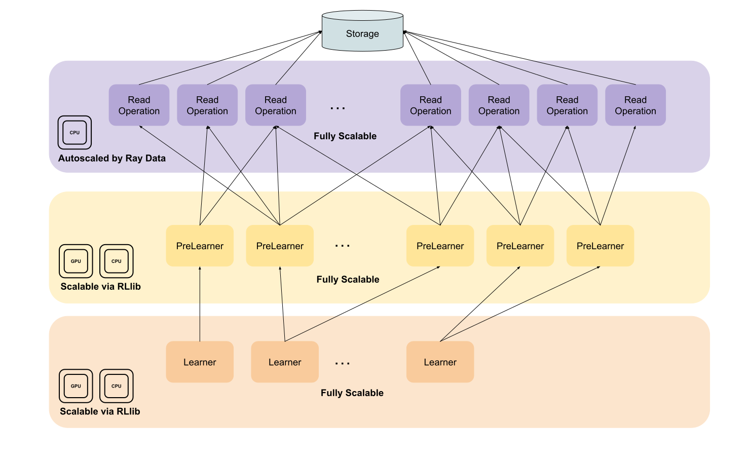
Read operations run exclusively on the CPU. Because Ray Data fully manages them, you scale them primarily by allocating additional resources. See How to tune performance for details. You scale post-processing by increasing the concurrency level in the keyword arguments for the mapping operation:
config = (
    AlgorithmConfig()
    .offline_data(
        map_batches_kwargs={
            "concurrency": 10,
            "num_cpus": 4,
        }
    )
)
This starts an actor pool with 10 DataWorker instances. Each runs an instance of RLlib’s callable OfflinePreLearner class to post-process batches for updating the RLModule.
Note
The num_cpus attribute, and likewise num_gpus, defines the resources allocated to each DataWorker, not to the full actor pool.
You scale the number of learners in RLlib’s learners() configuration block:
config = (
    AlgorithmConfig()
    .learners(
        num_learners=4,
        num_gpus_per_learner=1,
    )
)
With this configuration, you start an application with four remote Learner instances, each using a single GPU. See Learner (Alpha) for more about RLlib’s learners.
Using cloud storage#
Unlike RLlib’s old API stack, the offline RL API is cloud-agnostic and integrates with PyArrow. You can use any cloud storage path or PyArrow-compatible filesystem. If you use a PyArrow or compatible filesystem, make sure your input_ path is relative to that filesystem. As with Ray Data, you can use placeholders, lists of files or folders, or a single folder to read from recursively.
For example, to read from a storage bucket in GCS, you can specify the folder location as follows:
config=(
    AlgorithmConfig()
    .offline_data(
        input_="gs://<your-bucket>/dir1",
    )
)
With this configuration, RLlib reads data recursively from any folder beneath the specified path. If you use a filesystem for GCS, for instance because of authentication requirements, use the following syntax:
import pyarrow.fs

# Define the PyArrow filesystem
gcs = pyarrow.fs.GcsFilesystem(
    # This is needed to resolve the hostname for public buckets.
    anonymous=True,
    retry_time_limit=timedelta(seconds=15)
)

# Define the configuration.
config= (
    AlgorithmConfig()
    .offline_data(
        # NOTE: Use a relative file path now
        input_="<public-bucket>/dir1",
        input_filesystem=gcs,
    )
)
You can learn more about PyArrow’s filesystems, particularly regarding cloud filesystems and required authentication, in PyArrow Filesystem Interface.
Using cloud storage for recording#
You can use cloud storage in a similar way when recording experiences from an expert policy:
config= (
    AlgorithmConfig()
    .offline_data(
        output="gs://<your-bucket>/dir1",
    )
)
RLlib then writes directly into the folder in cloud storage, creating it in the bucket if it doesn’t exist. The only difference from reading is that you can’t use multiple paths for writing. For example, the following doesn’t work:
config= (
    AlgorithmConfig()
    .offline_data(
        output=["gs://<your-bucket>/dir1", "gs://<your-bucket>/dir2"],
    )
)
If the storage requires special permissions to create folders or write files, make sure the cluster user has those permissions. Otherwise, RLlib is denied write access and the recording process stops.
Note
When you use cloud storage, Ray Data typically streams data and consumes it in chunks, so post-processing and training begin after a brief warmup phase. Even if your cloud storage is large, the nodes running RLlib don’t need the same amount of space.
How to tune performance#
In RLlib’s offline RL API, distinct modules and configurations manage the key layers, which makes scaling these layers effectively non-trivial. Understand the specific parameters and their impact on system performance.
How to tune reading operations#
Ray Data handles and optimizes the Reading Operations layer automatically. Avoid modifying this process. A few parameters can improve performance on this layer somewhat:
Available resources dedicated to the job
Data locality
Data sharding
Data pruning
Available resources#
Ray Data’s scheduling strategy operates independently of any existing placement group and schedules tasks and actors separately. Reserve adequate resources for the other tasks and actors in your job. To improve read performance and Ray Data’s scalability for read operations, increase the available resources in your cluster while preserving the resource allocation for existing tasks and actors. Monitor and provision two key resources: CPUs and object store memory. Insufficient object store memory, especially under heavy backpressure, can spill objects to disk and severely degrade application performance.
Bandwidth strongly influences throughput within your cluster. In some cases, scaling the number of nodes increases bandwidth and improves the flow of data from storage to consuming processes. This approach helps in these scenarios:
Independent connections to the network backbone: nodes use dedicated bandwidth, which avoids shared uplinks and potential bottlenecks. See the AWS and GCP network bandwidth documentation.
Optimized cloud access: features such as S3 Transfer Acceleration, Google Cloud Storage FUSE, or parallel and accelerated data transfer methods improve performance.
Data locality#
Data locality is critical for fast data processing. For instance, if your data resides on GCP, running a Ray cluster on AWS S3 or a local machine results in low transfer rates and slow data processing. For efficient streaming with RLlib’s offline RL API, storing data in the same region, zone, and cloud provider as the Ray cluster is generally sufficient. Consider these additional adjustments:
Multi-region buckets: use multi-region storage to improve data availability and possibly increase access speeds for distributed systems.
Storage class optimization within buckets: use standard storage for frequent access and low-latency streaming. Avoid archival storage classes such as AWS Glacier or GCP Archive for streaming workloads, because of their high retrieval times.
Data sharding#
Data sharding improves the efficiency of fetching, transferring, and reading data by balancing chunk sizes. If chunks are too large, they can cause delays during transfer and processing, leading to bottlenecks. Conversely, chunks that are too small can result in high metadata fetching overhead, slowing down overall performance. Finding an optimal chunk size is critical for balancing these trade-offs and maximizing throughput.
As a rule of thumb, keep data file sizes between 64 MiB and 256 MiB.
Data pruning#
If your data is in Parquet format, the recommended offline data format for RLlib, you can use data pruning to optimize performance. Ray Data supports pruning in its read_parquet() method through projection pushdown, which filters columns, and filter pushdown, which filters rows. Ray Data applies these filters directly during file scans, which reduces the unnecessary data loaded into memory.
For instance, if you need only specific columns from your offline data, such as to avoid loading the infos column:
from ray.rllib.algorithms.algorithm_config import AlgorithmConfig
from ray.rllib.core.columns import Columns

config = (
    AlgorithmConfig()
    .offline_Data(
        input_read_method_kwargs={
            "columns": [
                Columns.EPS_ID,
                Columns.AGENT_ID,
                Columns.OBS,
                Columns.NEXT_OBS,
                Columns.REWARDS,
                Columns.ACTIONS,
                Columns.TERMINATED,
                Columns.TRUNCATED,
            ],
        },
    )
)
Similarly, if you need only specific rows from your dataset, apply pushdown filters as follows:
import pyarrow.dataset

from ray.rllib.algorithms.algorithm_config import AlgorithmConfig
from ray.rllib.core.columns import Columns

config = (
    AlgorithmConfig()
    .offline_data(
        input_read_method_kwargs={
            "filter": pyarrow.dataset.field(Columns.AGENT_ID) == "agent_1",
        },
    )
)
How to tune post-processing (PreLearner)#
When you enable high throughput in Read Operations, ensure sufficient processing capacity in the Post-Processing (Pre-Learner) stage. Insufficient capacity here can cause backpressure, which increases memory usage and, in severe cases, spills objects to disk or causes out-of-memory errors. See Out-Of-Memory Prevention.
Tuning the Post-Processing (Pre-Learner) layer is generally more straightforward than optimizing the Read Operations layer. You can adjust the following parameters to optimize its performance:
Actor pool size
Allocated resources
Read batch and buffer sizes
Actor pool size#
Internally, a map_batches() operation defines the Post-Processing (PreLearner) layer and starts an _ActorPool. Each actor in this pool runs an OfflinePreLearner instance to transform batches on their way from disk to RLlib’s Learner. The size of this _ActorPool determines the layer’s throughput, so fine-tune it against the previous layer’s throughput to avoid backpressure. Use concurrency in RLlib’s map_batches_kwargs parameter to define this pool size:
from ray.rllib.algorithm_config import AlgorithmConfig

config = (
    AlgorithmConfig()
    .offline_data(
        map_batches_kwargs={
            "concurrency": 4,
        },
    )
)
With the preceding code, Ray Data starts up to 4 parallel OfflinePreLearner actors that post-process your data for training.
Note
Ray Data adjusts its read operations dynamically based on the parallelism of your Post-Processing (Pre-Learner) layer, scaling them up or down depending on the backpressure in that stage. So the performance of the downstream tasks and the resources allocated to the Reading Operations layer determine the throughput of your entire streaming pipeline. See How to tune reading operations. Because scaling reading operations up or down carries overhead, you can’t always avoid backpressure entirely, or object spilling and out-of-memory (OOM) errors in severe cases.
You can also enable auto-scaling in your Post-Processing (PreLearner) by providing an interval instead of a straight number:
from ray.rllib.algorithm_config import AlgorithmConfig

config = (
    AlgorithmConfig()
    .offline_data(
        map_batches_kwargs={
            "concurrency": (4, 8),
        },
    )
)
With this, Ray Data starts up to 8 post-processing actors to move data downstream faster, for example under backpressure.
Note
An autoscaled actor pool in the Post-Processing (Pre-Learner) layer doesn’t guarantee that backpressure disappears. Adding more OfflinePreLearner instances introduces overhead. RLlib’s offline RL pipeline is optimized for streaming data, which typically shows stable throughput and resource usage, except when upstream and downstream tasks are imbalanced. As a rule of thumb, use autoscaling only when one of the following holds:
Throughput is highly variable.
Cluster resources fluctuate, for example in shared or dynamic environments.
Workload characteristics are highly unpredictable.
Allocated resources#
Besides the number of post-processing actors, you can tune the Post-Processing (PreLearner) layer by defining the resources allocated to each OfflinePreLearner in the actor pool. Define these resources through num_cpus and num_gpus, or in ray_remote_args.
Note
Typically, increasing the number of CPUs is enough to tune the post-processing stage. You need GPUs only in specialized cases, such as customized pipelines. For example, RLlib’s MARWIL implementation uses the GeneralAdvantageEstimation connector in its ConnectorPipelineV2 to apply General Advantage Estimation to experience batches. These calculations apply the value model of the algorithm’s RLModule, which you can accelerate by running on a GPU.
For example, to give each of your 4 OfflinePreLearner instances in the Post-Processing (PreLearner) layer 2 CPUs, use the following syntax:
from ray.rllib.algorithms.algorithm_config import AlgorithmConfig

config = (
    AlgorithmConfig()
    .offline_data(
        map_batches_kwargs={
            "concurrency": 4,
            "num_cpus": 2,
        },
    )
)
Warning
Don’t override the batch_size in RLlib’s map_batches_kwargs. Doing so usually degrades performance significantly. This batch_size differs from train_batch_size_per_learner. The former sets the batch size for transformations in the streaming pipeline. The latter sets the batch size for training within each Learner, the batch size of the model forward and backward passes performed for training.
Read batch and buffer sizes#
When you work with data from SingleAgentEpisode or the legacy SampleBatch format, fine-tuning the input_read_batch_size parameter gives you more optimization opportunities. This parameter controls the size of batches retrieved from data files. It matters most for episodic or legacy SampleBatch data, because for that data the streaming pipeline uses an EpisodeReplayBuffer to handle the multiple timesteps in each data row. RLlib converts all incoming data into SingleAgentEpisode instances, if it isn’t already in that format, and stores it in an episode replay buffer, which precisely manages the sampling of train_batch_size_per_learner for training.
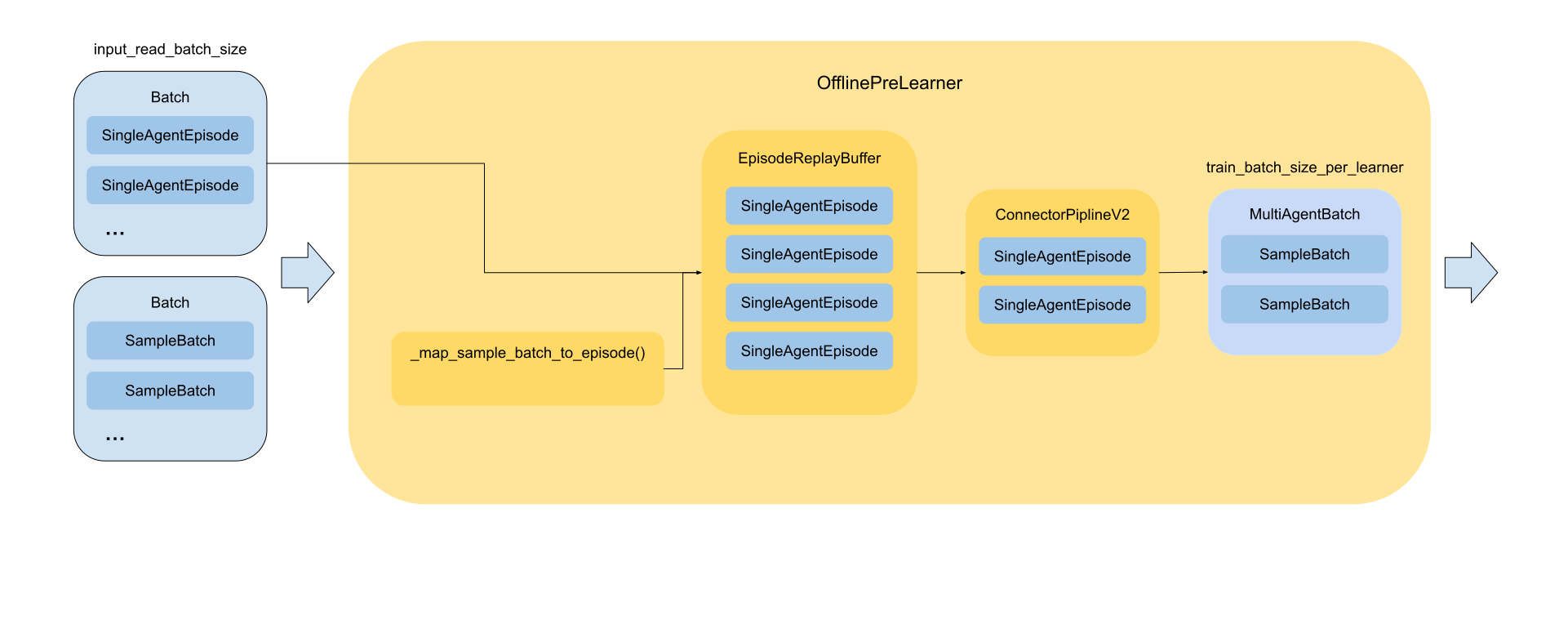
An optimal balance between data ingestion efficiency and sampling variation in your streaming pipeline is crucial. Consider an example. Suppose each SingleAgentEpisode has a length of 100 timesteps, and you configure train_batch_size_per_learner to 1000. Each EpisodeReplayBuffer instance has a capacity of 1000:
from ray.rllib.algorithms.algorithm_config import AlgorithmConfig

config = (
    AlgorithmConfig()
    .training(
        # Train on a batch of 1000 timesteps each iteration.
        train_batch_size_per_learner=1000,
    )
    .offline_data(
        # Read in RLlib's new stack `SingleAgentEpisode` data.
        input_read_episodes=True
        # Define an input read batch size of 10 episodes.
        input_read_batch_size=10,
        # Set the replay buffer in the `OfflinePrelearner`
        # to 1,000 timesteps.
        prelearner_buffer_kwargs={
            "capacity": 1000,
        },
    )
)
If you configure input_read_batch_size to 10 as shown in the code, all 10 SingleAgentEpisode instances fit into the buffer, so you can sample across a wide variety of timesteps from multiple episodes. This produces high sampling variation. Next, consider a buffer capacity reduced to 500:
from ray.rllib.algorithms.algorithm_config import AlgorithmConfig

config = (
    AlgorithmConfig()
    .training(
        # Train on a batch of 1000 timesteps each iteration.
        train_batch_size_per_learner=1000,
    )
    .offline_data(
        # Read in RLlib's new stack `SingleAgentEpisode` data.
        input_read_episodes=True
        # Define an input read batch size of 10 episodes.
        input_read_batch_size=10,
        # Set the replay buffer in the `OfflinePrelearner`
        # to 500 timesteps.
        prelearner_buffer_kwargs={
            "capacity": 500,
        },
    )
)
With the same input_read_batch_size, the buffer holds only 5 SingleAgentEpisode instances at a time, which causes inefficiency because RLlib reads more data than it can retain for sampling.
In another scenario, each SingleAgentEpisode still has a length of 100 timesteps, and you set train_batch_size_per_learner to 4000 timesteps as in the following code. The buffer holds 10 SingleAgentEpisode instances. This configuration produces lower sampling variation, because RLlib samples many timesteps repeatedly, which reduces diversity across training batches. These examples show why tuning these parameters to balance data ingestion and sampling diversity in your offline streaming pipeline matters.
from ray.rllib.algorithms.algorithm_config import AlgorithmConfig

config = (
    AlgorithmConfig()
    .training(
        # Train on a batch of 4000 timesteps each iteration.
        train_batch_size_per_learner=4000,
    )
    .offline_data(
        # Read in RLlib's new stack `SingleAgentEpisode` data.
        input_read_episodes=True
        # Define an input read batch size of 10 episodes.
        input_read_batch_size=10,
        # Set the replay buffer in the `OfflinePrelearner`
        # to 1,000 timesteps.
        prelearner_buffer_kwargs={
            "capacity": 500,
        },
    )
)
Tip
To choose an appropriate input_read_batch_size, look at the length of your recorded episodes. In some cases, a single episode is long enough to fill train_batch_size_per_learner, and you can choose an input_read_batch_size of 1. Most of the time it isn’t, so consider how many episodes to buffer to balance the data digested from read input against the variation of data sampled from the EpisodeReplayBuffer instances in the OfflinePreLearner.
How to tune updating (Learner)#
Updating (Learner) is the final downstream task in RLlib’s Offline RL pipeline, and its consumption speed determines the overall throughput of the data pipeline. If the learning process is slow, it can cause backpressure in upstream layers and potentially spill objects or cause out-of-memory (OOM) errors. Fine-tune this layer together with the upstream components. You can adjust several parameters to optimize the learning speed in your offline algorithm:
Actor pool size
Allocated resources
Scheduling strategy
Batch sizing
Batch prefetching
Learner iterations
Actor pool size#
RLlib scales Learner instances through the num_learners parameter. When this value is 0, RLlib uses a Learner instance in the local process. For values greater than 0, RLlib scales out with a BackendExecutor. This executor spawns your specified number of Learner instances, manages distributed training, and aggregates intermediate results across Learner actors. Scaling Learner instances increases training throughput. Apply it only when the upstream components in your Offline Data pipeline can supply data fast enough to match the increased training capacity. RLlib’s Offline API scales at its final layer with streaming_split, which divides the data stream into multiple substreams. Individual Learner instances then process these substreams, which enables efficient parallel consumption and improves overall throughput.
For example, to set the number of learners to 4, use the following syntax:
from ray.rllib.algorithms.algorithm_config import AlgorithmConfig

config = (
    AlgorithmConfig()
    .learners(num_learners=4)
)
Allocated resources#
As with the Post-Processing (Pre-Learner) layer, allocating additional resources can help with slow training. The primary resource is the GPU, because training involves forward and backward passes through the RLModule, which GPUs accelerate significantly. If your training already uses GPUs and performance remains an issue, scale up in one of two ways. Add more GPUs to each Learner to increase GPU memory and computational capacity with config.learners(num_gpus_per_learner=...), or add more Learner workers to distribute the workload further with config.learners(num_learners=...). Also ensure that data throughput and upstream components are optimized to keep the learners fully used, because insufficient upstream capacity can bottleneck training.
Warning
You can’t set both num_gpus_per_learner and num_cpus_per_learner, because of placement group fragmentation in Ray.
To give your learners more compute, use num_gpus_per_learner or num_cpus_per_learner as follows:
from ray.rllib.algorithms.algorithm_config import AlgorithmConfig

config = (
    AlgorithmConfig()
    .learners(num_learners=4, num_gpus_per_learner=2)
)
Tip
If you experience backpressure in the Post-Processing (Pre-Learner) stage, enable GPU training before you scale up the number of Learner instances.
Scheduling strategy#
The scheduling strategy in Ray plays a key role in task and actor placement. It tries to distribute tasks and actors across multiple nodes in a cluster to maximize resource utilization and fault tolerance. On a single-node cluster, one large head node, the scheduling strategy has little to no noticeable impact. In a multi-node cluster, scheduling can significantly influence the performance of your Offline Data pipeline, because data locality matters. Data processing occurs across all nodes, and maintaining data locality during training can improve performance.
In such scenarios, you can improve data locality by changing RLlib’s default scheduling strategy from "PACK" to "SPREAD". This strategy distributes the Learner actors across the cluster, so Ray Data can use locality-aware bundle selection to improve efficiency.
The following example changes the scheduling strategy:
"""Just for show-casing, don't run."""
import os
from ray import data
from ray.rllib.algorithms.algorithm_config.AlgorithmConfig

# Configure a "SPREAD" scheduling strategy for learners.
os.environ["TRAIN_ENABLE_WORKER_SPREAD_ENV"] = "1"

# Get the current data context.
data_context = data.DataContext.get_current()
# Configure the Ray Data scheduling strategy used by the offline pipeline.
data_context.scheduling_strategy = "SPREAD"

# Build the config.
config = (
    AlgorithmConfig()
    .learners(
        # Scale the learners.
        num_learners=4,
        num_gpus_per_learner=2,
    )
    .offline_data(
        ...,
        # Run in each RLlib training iteration 10
        # iterations per learner (each of them with
        # `train_batch_size_per_learner`).
        dataset_num_iters_per_learner=20,
    )
)

# Build the algorithm from the config.
algo = config.build()

# Train for 10 iterations.
for _ in range(10)
    res = algo.train()
Warning
Changing scheduling strategies in RLlib’s offline RL API is experimental. Use it with caution.
Batch size#
Batch size is one of the simplest parameters to adjust when you optimize performance in RLlib’s offline RL API. Small batch sizes can under-use hardware and create inefficiencies, and overly large batch sizes can exceed memory limits. In a streaming pipeline, the batch size you select affects how RLlib partitions and processes data across parallel workers. Larger batch sizes reduce the overhead of frequent task coordination, but if they exceed hardware constraints, they can slow down the entire pipeline. Configure the training batch size with the train_batch_size_per_learner attribute as follows.
from ray.rllib.algorithms.algorithm_config import AlgorithmConfig

config = (
    AlgorithmConfig()
    .training(
        train_batch_size_per_learner=1024,
    )
)
Tip
A good starting point for batch size tuning is 2048.
In Ray Data, it’s common to use batch sizes that are powers of two. You can select any integer value for the batch size based on your needs.
Batch prefetching#
Batch prefetching controls data consumption on the downstream side of your offline data pipeline. The goal is to keep learners active and maintain a continuous flow of data. RLlib prepares the next batch while the learner processes the current one. Prefetching determines how many batches RLlib keeps ready for learners. Tune it based on the time needed to produce the next batch and the learner’s update speed. Prefetching too many batches can cause memory inefficiencies and, in some cases, backpressure in upstream tasks.
Tip
The default in RLlib’s Offline RL API is to prefetch 2 batches per learner instance, which works well with most tested applications.
You can configure batch prefetching in the iter_batches_kwargs:
from ray.rllib.algorithms.algorithm_config import AlgorithmConfig

config = (
    AlgorithmConfig()
    .offline_data(
        iter_batches_kwargs={
            "prefetch_batches": 2,
        }
    )
)
Warning
Don’t override the batch_size in RLlib’s map_batches_kwargs. Doing so usually degrades performance significantly. This batch_size differs from train_batch_size_per_learner. The former sets the batch size for iterating over the data output of the streaming pipeline. The latter sets the batch size for training within each Learner.
Learner iterations#
This tuning parameter is available only when you use multiple Learner instances. In distributed learning, each Learner instance processes a sub-stream of the offline streaming pipeline and iterates over batches from that sub-stream. You can control the number of iterations each Learner instance runs per RLlib training iteration. Result reporting occurs after each RLlib training iteration. Setting this parameter too low creates inefficiencies. Setting it too high can hinder training monitoring and, in some cases, such as RLlib’s MARWIL implementation, lead to stale training data. This happens because some data transformations rely on the same RLModule that the Learner instances train on. The attribute dataset_num_iters_per_learner controls the number of iterations per sub-stream. Its default value is None, which runs one epoch on the sub-stream.
You can modify this value as follows:
from ray.rllib.algorithms.algorithm_config import AlgorithmConfig

config = (
    AlgorithmConfig()
    .offline_data(
        # Train on 20 batches from the substream in each learner.
        dataset_num_iters_per_learner=20,
    )
)
Note
The default value of dataset_num_iters_per_learner is None, so each Learner instance processes a full epoch on its data substream. This setting works well for small datasets but might not suit larger ones. Tune this parameter according to the size of your dataset for optimal performance.
Customization#
Customizing the Offline RL components in RLlib, such as the Algorithm, Learner, or RLModule, follows a similar process to their Online RL counterparts. For detailed guidance, see the documentation on Algorithms, Learners, and RLlib’s RLModule. RLlib’s Offline RL streaming pipeline supports customization at three levels, so you can tailor it to your offline RL algorithm:
Connector level
PreLearner level
Pipeline level
Connector level#
You can implement small data transformations on SingleAgentEpisode instances by modifying the ConnectorPipelineV2, which is part of the OfflinePreLearner and prepares episodes for training. Use any connector from RLlib’s library, listed in RLlib’s default connectors, or create a custom connector, shown in RLlib’s ConnectorV2 examples, to integrate into the Learner’s ConnectorPipelineV2. Consider the order in which RLlib applies ConnectorV2 instances carefully, as the implementation of RLlib’s MARWIL algorithm demonstrates. See the MARWIL paper.
The MARWIL algorithm computes a loss that extends beyond behavior cloning by improving the expert’s strategy during training with advantages. RLlib calculates these advantages through General Advantage Estimation (GAE) with a value model. It computes GAE on the fly through the GeneralAdvantageEstimation connector. This connector has specific requirements. It processes a list of SingleAgentEpisode instances and must be one of the final components in the ConnectorPipelineV2, because it relies on fully prepared batches that contain OBS, REWARDS, NEXT_OBS, TERMINATED, and TRUNCATED fields. The incoming SingleAgentEpisode instances must also already include one artificially elongated timestep.
To meet these requirements, the pipeline must include the following sequence of ConnectorV2 instances:
ray.rllib.connectors.learner.add_one_ts_to_episodes_and_truncate.AddOneTsToEpisodesAndTruncateelongates theSingleAgentEpisodeobjects by one timestep.ray.rllib.connectors.common.add_observations_from_episodes_to_batch.AddObservationsFromEpisodesToBatchincorporates the observations,OBS, into the batch.ray.rllib.connectors.learner.add_next_observations_from_episodes_to_train_batch.AddNextObservationsFromEpisodesToTrainBatchadds the next observations,NEXT_OBS.Finally, RLlib applies the
ray.rllib.connectors.learner.general_advantage_estimation.GeneralAdvantageEstimationconnector piece.
The following code snippet from RLlib’s MARWIL algorithm demonstrates this setup:
@override(AlgorithmConfig)
def build_learner_connector(
    self,
    input_observation_space,
    input_action_space,
    device=None,
):
    pipeline = super().build_learner_connector(
        input_observation_space=input_observation_space,
        input_action_space=input_action_space,
        device=device,
    )

    # Before anything, add one ts to each episode (and record this in the loss
    # mask, so that the computations at this extra ts aren't used to compute
    # the loss).
    pipeline.prepend(AddOneTsToEpisodesAndTruncate())

    # Prepend the "add-NEXT_OBS-from-episodes-to-train-batch" connector piece (right
    # after the corresponding "add-OBS-..." default piece).
    pipeline.insert_after(
        AddObservationsFromEpisodesToBatch,
        AddNextObservationsFromEpisodesToTrainBatch(),
    )

    # At the end of the pipeline (when the batch is already completed), add the
    # GAE connector, which performs a vf forward pass, then computes the GAE
    # computations, and puts the results of this (advantages, value targets)
    # directly back in the batch. This is then the batch used for
    # `forward_train` and `compute_losses`.
    pipeline.append(
        GeneralAdvantageEstimation(gamma=self.gamma, lambda_=self.lambda_)
    )

    return pipeline
Define a primer LearnerConnector pipeline#
You can customize the LearnerConnectorPipeline in several ways. One approach, shown earlier, is to override the build_learner_connector method in the Algorithm. Alternatively, you can define a custom ConnectorV2 piece for the LearnerConnectorPipeline with the learner_connector attribute:
def _make_learner_connector(input_observation_space, input_action_space):
    # Create the learner connector.
    return CustomLearnerConnector(
        parameter_1=0.3,
        parameter_2=100,
    )

config = (
    AlgorithmConfig()
    .training(
        # Add the connector pipeline as the starting point for
        # the learner connector pipeline.
        learner_connector=_make_learner_connector,
    )
)
As the comments note, this approach to adding a ConnectorV2 piece to the LearnerConnectorPipeline is suitable only if you intend to manipulate raw episodes, because your ConnectorV2 piece is the foundation for building the rest of the pipeline, including batching and other processing steps. If you want to modify data further along in the LearnerConnectorPipeline, either override the Algorithm’s build_learner_connector method or use the third option, overriding the entire PreLearner.
PreLearner level#
If you need to perform data transformations at a deeper level, before your data reaches the SingleAgentEpisode stage, override the OfflinePreLearner. This class orchestrates the complete data transformation pipeline and converts raw input data into MultiAgentBatch objects ready for training. For instance, if your data is in specialized formats that need pre-parsing and restructuring, such as XML, HTML, Protobuf, images, or videos, you might need to handle these custom formats directly. You can use tools such as Ray Data’s custom datasources, for example read_binary_files(), to manage the ingestion. To structure and sort this data into SingleAgentEpisode objects, override the _map_to_episodes() static method.
For more extensive customization, you can rewrite the __call__ method to define custom transformation steps, implement a unique LearnerConnectorPipeline, and construct MultiAgentBatch instances for the Learner.
The following example demonstrates how to use a custom OfflinePreLearner to process text data and construct training batches:
import gymnasium as gym
import numpy as np
import uuid
from typing import Any, Dict, List, Optional, Union

from ray import data
from ray.rllib.env.single_agent_episode import SingleAgentEpisode
from ray.rllib.offline.offline_prelearner import OfflinePreLearner, SCHEMA
from ray.rllib.utils.annotations import override
from ray.rllib.utils.typing import EpisodeType

class TextOfflinePreLearner(OfflinePreLearner):

    @staticmethod
    @override(OfflinePreLearner)
    def _map_to_episodes(
        is_multi_agent: bool,
        batch: Dict[str, Union[list, np.ndarray]],
        schema: Dict[str, str] = SCHEMA,
        to_numpy: bool = False,
        input_compress_columns: Optional[List[str]] = None,
        observation_space: gym.Space = None,
        action_space: gym.Space = None,
        vocabulary: Dict[str, Any] = None,
        **kwargs: Dict[str, Any],
    ) -> Dict[str, List[EpisodeType]]:

        # If we have no vocabulary raise an error.
        if not vocabulary:
            raise ValueError(
                "No `vocabulary`. It needs a vocabulary in form of dictionary ",
                "mapping tokens to their IDs."
            )
        # Define container for episodes.
        episodes = []

        # Data comes in batches of string arrays under the `"text"` key.
        for text in batch["text"]:
            # Split the text and tokenize.
            tokens = text.split(" ")
            # Encode tokens.
            encoded = [vocabulary[token] for token in tokens]
            one_hot_vectors = np.zeros((len(tokens), len(vocabulary), 1, 1))
            for i, token in enumerate(tokens):
                if token in vocabulary:
                    one_hot_vectors[i][vocabulary[token] - 1] = 1.0

            # Build the `SingleAgentEpisode`.
            episode = SingleAgentEpisode(
                # Generate a unique ID.
                id_=uuid.uuid4().hex,
                # agent_id="default_policy",
                # module_id="default_policy",
                # We use the starting token with all added tokens as observations.
                observations=[ohv for ohv in one_hot_vectors],
                observation_space=observation_space,
                # Actions are defined to be the "chosen" follow-up token after
                # given the observation.
                actions=encoded[1:],
                action_space=action_space,
                # Rewards are zero until the end of a sequence.
                rewards=[0.0 for i in range(len(encoded) - 2)] + [1.0],
                # The episode is always terminated (as sentences in the dataset are).
                terminated=True,
                truncated=False,
                # No lookback. You want the episode to start at timestep zero.
                len_lookback_buffer=0,
                t_started=0,
            )

            # If episodes should be numpy'ized. Some connectors need this.
            if to_numpy:
                episode.to_numpy()

            # Append the episode to the list of episodes.
            episodes.append(episode)

        # Return a batch with key `"episodes"`.
        return {"episodes": episodes}

# Define the dataset.
ds = data.read_text("s3://anonymous@ray-example-data/this.txt")

# Create a vocabulary.
tokens = []
for b in ds.iter_rows():
    tokens.extend(b["text"].split(" "))
vocabulary = {token: idx for idx, token in enumerate(set(tokens), start=1)}

# Take a small batch of 10 from the dataset.
batch = ds.take_batch(10)

# Now use your `OfflinePreLearner`.
episodes = TextOfflinePreLearner._map_to_episodes(
    is_multi_agent=False,
    batch=batch,
    to_numpy=True,
    schema=None,
    input_compress_columns=False,
    action_space=None,
    observation_space=None,
    vocabulary=vocabulary,
)

# Show the constructed episodes.
print(f"Episodes: {episodes}")
The preceding example illustrates the flexibility of RLlib’s Offline RL API for custom data transformation. Here, a customized OfflinePreLearner processes a batch of text data, organized as sentences, and converts each sentence into a SingleAgentEpisode. The static method returns a dictionary that contains a list of these SingleAgentEpisode instances. You can extend this behavior by overriding the __call__() method. For instance, you could implement a ray.rllib.connectors.learner.learner_connector_pipeline.LearnerConnectorPipeline that stacks multiple observations, such as tokens, together. RLlib’s FrameStackingLearner does this, as the following example shows.
import gymnasium as gym
import numpy as np
import uuid
from typing import Any, Dict, List, Optional, Tuple, Union

from ray import data
from ray.actor import ActorHandle
from ray.rllib.algorithms.algorithm_config import AlgorithmConfig
from ray.rllib.algorithms.bc.bc_catalog import BCCatalog
from ray.rllib.algorithms.bc.torch.default_bc_torch_rl_module import DefaultBCTorchRLModule
from ray.rllib.connectors.common import AddObservationsFromEpisodesToBatch, BatchIndividualItems, NumpyToTensor, AgentToModuleMapping
from ray.rllib.connectors.learner.add_columns_from_episodes_to_train_batch import AddColumnsFromEpisodesToTrainBatch
from ray.rllib.connectors.learner.frame_stacking import FrameStackingLearner
from ray.rllib.connectors.learner.learner_connector_pipeline import LearnerConnectorPipeline
from ray.rllib.core.learner.learner import Learner
from ray.rllib.core.rl_module.default_model_config import DefaultModelConfig
from ray.rllib.core.rl_module.multi_rl_module import MultiRLModuleSpec
from ray.rllib.core.rl_module.rl_module import RLModuleSpec
from ray.rllib.env.single_agent_episode import SingleAgentEpisode
from ray.rllib.policy.sample_batch import MultiAgentBatch, SampleBatch
from ray.rllib.offline.offline_prelearner import OfflinePreLearner, SCHEMA

from ray.rllib.utils.annotations import override
from ray.rllib.utils.typing import EpisodeType, ModuleID

class TextOfflinePreLearner(OfflinePreLearner):

    @override(OfflinePreLearner)
    def __init__(
        self,
        config: "AlgorithmConfig",
        learner: Union[Learner, List[ActorHandle]] = None,
        locality_hints: Optional[List[str]] = None,
        spaces: Optional[Tuple[gym.Space, gym.Space]] = None,
        module_spec: Optional[MultiRLModuleSpec] = None,
        module_state: Optional[Dict[ModuleID, Any]] = None,
        vocabulary: Dict[str, Any] = None,
        **kwargs: Dict[str, Any],
    ):
        self.config = config
        self.spaces = spaces
        self.vocabulary = vocabulary
        self.vocabulary_size = len(self.vocabulary)

        # Build the `RLModule`.
        self._module = module_spec.build()
        if module_state:
            self._module.set_state(module_state)

        # Build the learner connector pipeline.
        self._learner_connector = LearnerConnectorPipeline(
            connectors=[
                FrameStackingLearner(
                    num_frames=4,
                )
            ],
            input_action_space=module_spec.action_space,
            input_observation_space=module_spec.observation_space,
        )
        self._learner_connector.append(
            AddObservationsFromEpisodesToBatch(as_learner_connector=True),
        )
        self._learner_connector.append(
            AddColumnsFromEpisodesToTrainBatch(),
        )
        self._learner_connector.append(
            BatchIndividualItems(multi_agent=False),
        )
        # Let us run exclusively on CPU, then we can convert here to Tensor.
        self._learner_connector.append(
            NumpyToTensor(as_learner_connector=True),
        )

    @override(OfflinePreLearner)
    def __call__(self, batch: Dict[str, np.ndarray]) -> Dict[str, List[EpisodeType]]:

        # Convert raw data to episodes.
        episodes = TextOfflinePreLearner._map_to_episodes(
            is_multi_agent=False,
            batch=batch,
            to_numpy=True,
            schema=None,
            input_compress_columns=False,
            action_space=self.spaces[0],
            observation_space=self.spaces[1],
            vocabulary=self.vocabulary,
        )["episodes"]

        # Run the learner connector pipeline with the
        # `FrameStackLearner` piece.
        batch = self._learner_connector(
            rl_module=self._module,
            batch={},
            episodes=episodes,
            shared_data={},
        )

        # Convert to `MultiAgentBatch` for the learner.
        batch = MultiAgentBatch(
            {
                module_id: SampleBatch(module_data)
                for module_id, module_data in batch.items()
            },
            # TODO (simon): This can be run once for the batch and the
            # metrics, but we run it twice: here and later in the learner.
            env_steps=sum(e.env_steps() for e in episodes),
        )

        # Return the `MultiAgentBatch` under the `"batch"` key.
        return {"batch": batch}

    @staticmethod
    @override(OfflinePreLearner)
    def _map_to_episodes(
        is_multi_agent: bool,
        batch: Dict[str, Union[list, np.ndarray]],
        schema: Dict[str, str] = SCHEMA,
        to_numpy: bool = False,
        input_compress_columns: Optional[List[str]] = None,
        observation_space: gym.Space = None,
        action_space: gym.Space = None,
        vocabulary: Dict[str, Any] = None,
        **kwargs: Dict[str, Any],
    ) -> Dict[str, List[EpisodeType]]:

        # If we have no vocabulary raise an error.
        if not vocabulary:
            raise ValueError(
                "No `vocabulary`. It needs a vocabulary in form of dictionary ",
                "mapping tokens to their IDs."
            )
        # Define container for episodes.
        episodes = []

        # Data comes in batches of string arrays under the `"text"` key.
        for text in batch["text"]:
            # Split the text and tokenize.
            tokens = text.split(" ")
            # Encode tokens.
            encoded = [vocabulary[token] for token in tokens]
            one_hot_vectors = np.zeros((len(tokens), len(vocabulary), 1, 1))
            for i, token in enumerate(tokens):
                if token in vocabulary:
                    one_hot_vectors[i][vocabulary[token] - 1] = 1.0

            # Build the `SingleAgentEpisode`.
            episode = SingleAgentEpisode(
                # Generate a unique ID.
                id_=uuid.uuid4().hex,
                # agent_id="default_policy",
                # module_id="default_policy",
                # We use the starting token with all added tokens as observations.
                observations=[ohv for ohv in one_hot_vectors],
                observation_space=observation_space,
                # Actions are defined to be the "chosen" follow-up token after
                # given the observation.
                actions=encoded[1:],
                action_space=action_space,
                # Rewards are zero until the end of a sequence.
                rewards=[0.0 for i in range(len(encoded) - 2)] + [1.0],
                # The episode is always terminated (as sentences in the dataset are).
                terminated=True,
                truncated=False,
                # No lookback. You want the episode to start at timestep zero.
                len_lookback_buffer=0,
                t_started=0,
            )

            # If episodes should be numpy'ized. Some connectors need this.
            if to_numpy:
                episode.to_numpy()

            # Append the episode to the list of episodes.
            episodes.append(episode)

        # Return a batch with key `"episodes"`.
        return {"episodes": episodes}

# Define dataset on sample data.
ds = data.read_text("s3://anonymous@ray-example-data/this.txt")

# Create a vocabulary.
tokens = []
for b in ds.iter_rows():
    tokens.extend(b["text"].split(" "))
vocabulary = {token: idx for idx, token in enumerate(set(tokens), start=1)}

# Specify an `RLModule` and wrap it with a `MultiRLModuleSpec`. Note,
# on `Learner`` side any `RLModule` is an `MultiRLModule`.
module_spec = MultiRLModuleSpec(
    rl_module_specs={
        "default_policy": RLModuleSpec(
            model_config=DefaultModelConfig(
                conv_filters=[[16, 4, 2], [32, 4, 2], [64, 4, 2], [128, 4, 2]],
                conv_activation="relu",
            ),
            inference_only=False,
            module_class=DefaultBCTorchRLModule,
            catalog_class=BCCatalog,
            action_space = gym.spaces.Discrete(len(vocabulary)),
            observation_space=gym.spaces.Box(0.0, 1.0, (len(vocabulary), 1, 1), np.float32),
        ),
    },
)

# Take a small batch.
batch = ds.take_batch(10)

# Build and instance your `OfflinePreLearner`.
oplr = TextOfflinePreLearner(
    config=AlgorithmConfig(),
    spaces=(
        gym.spaces.Discrete(len(vocabulary)),
        gym.spaces.Box(0.0, 1.0, (len(vocabulary), 1, 1), np.float32)),
    module_spec=module_spec,
    vocabulary=vocabulary,
)

# Run your `OfflinePreLearner`.
transformed = oplr(batch)

# Show the generated batch.
print(f"Batch: {batch}")
Fully customizing the OfflinePreLearner gives you tailored data transformation workflows. You can define a specific learner connector pipeline and implement raw data mapping, which processes text data in multiple steps from its raw format to a MultiAgentBatch.
To integrate your custom OfflinePreLearner, specify it in your AlgorithmConfig:
from ray.rllib.algorithms.algorithm_config import AlgorithmConfig

config = (
    AlgorithmConfig()
    .offline_data(
        # Provide your custom `OfflinePreLearner`.
        prelearner_class=TextOfflinePreLearner,
        # Provide special keyword arguments your `OfflinePreLearner` needs.
        prelearner_kwargs={
            "vocabulary": vocabulary,
        },
    )
)
If these customization capabilities still don’t meet your requirements, move to the Pipeline Level for greater flexibility.
Pipeline level#
At this level of RLlib’s Offline RL API, you can redefine your complete pipeline from data reading to batch iteration by overriding the OfflineData class. In most cases, though, the other two levels are sufficient. Manipulating the complete pipeline needs careful handling, because it can degrade your pipeline’s performance significantly. Study the OfflineData class carefully to understand how the default pipeline works before you program your own. Two main methods define this pipeline:
The
__init__()method that defines the data reading process.The
sample()method that defines the data mapping and batch iteration.
For example, consider overriding the __init__() method if you have foundational data transformations, such as transforming image files into NumPy arrays.
import io
import logging
from typing import Any, Dict

import numpy as np
from PIL import Image

from ray import data
from ray.rllib.algorithms.algorithm_config import AlgorithmConfig
from ray.rllib.offline.offline_data import OfflineData
from ray.rllib.offline.offline_prelearner import OfflinePreLearner
from ray.rllib.utils.annotations import override

logger = logging.getLogger(__name__)


class ImageOfflineData(OfflineData):
    """This class overrides `OfflineData` to read in raw image data.

    The image data is from Ray Data`s S3 example bucket, namely
    `ray-example-data/batoidea/JPEGImages/`.
    To read in this data the raw bytes have to be decoded and then
    converted to `numpy` arrays. Each image array has a dimension
    (32, 32, 3).

    To just read in the raw image data and convert it to arrays it
    suffices to override the `OfflineData.__init__` method only.
    Note, that further transformations of the data - specifically
    into `SingleAgentEpisode` data - will be performed in a custom
    `OfflinePreLearner` defined in the `image_offline_prelearner`
    file. You could hard-code the usage of this prelearner here,
    but you will use the `prelearner_class` attribute in the
    `AlgorithmConfig` instead.
    """

    @override(OfflineData)
    def __init__(self, config: AlgorithmConfig):

        # Set class attributes.
        self.config = config
        self.is_multi_agent = self.config.is_multi_agent
        self.materialize_mapped_data = False
        self.path = self.config.input_

        self.data_read_batch_size = self.config.input_read_batch_size
        self.data_is_mapped = False

        # Define your function to map images to numpy arrays.
        def map_to_numpy(row: Dict[str, Any]) -> Dict[str, Any]:
            # Convert to byte stream.
            bytes_stream = io.BytesIO(row["bytes"])
            # Convert to image.
            image = Image.open(bytes_stream)
            # Return an array of the image.
            return {"array": np.array(image)}

        try:
            # Load the dataset and transform to arrays on-the-fly.
            self.data = data.read_binary_files(self.path).map(map_to_numpy)
        except Exception as e:
            logger.error(e)

        # Define further attributes needed in the `sample` method.
        self.batch_iterator = None
        self.map_batches_kwargs = self.config.map_batches_kwargs
        self.iter_batches_kwargs = self.config.iter_batches_kwargs
        # Use a custom OfflinePreLearner if needed.
        self.prelearner_class = self.config.prelearner_class or OfflinePreLearner

        # For remote learner setups.
        self.locality_hints = None
        self.learner_handles = None
        self.module_spec = None
In the preceding code example, you define a custom OfflineData class to handle reading and preprocessing image data and convert it from a binary encoding format into numpy arrays. You then implement a custom OfflinePreLearner to process this data further and transform it into a learner-ready MultiAgentBatch format.
import random
import uuid
from typing import Any, Dict, List, Optional, Tuple, Union

import gymnasium as gym
import numpy as np

from ray.actor import ActorHandle
from ray.rllib.algorithms.algorithm_config import AlgorithmConfig
from ray.rllib.core.learner.learner import Learner
from ray.rllib.core.rl_module.multi_rl_module import MultiRLModuleSpec
from ray.rllib.env.single_agent_episode import SingleAgentEpisode
from ray.rllib.offline.offline_prelearner import SCHEMA, OfflinePreLearner
from ray.rllib.utils.annotations import override
from ray.rllib.utils.typing import EpisodeType, ModuleID


class ImageOfflinePreLearner(OfflinePreLearner):
    """This class transforms image data to `MultiAgentBatch`es.

    While the `ImageOfflineData` class transforms raw image
    bytes to `numpy` arrays, this class maps these data in
    `SingleAgentEpisode` instances through the learner connector
    pipeline and finally outputs a >`MultiAgentBatch` ready for
    training in RLlib's `Learner`s.

    Note, the basic transformation from images to `SingleAgentEpisode`
    instances creates synthetic data that does not rely on any MDP
    and therefore no agent can learn from it. However, this example
    should show how to transform data into this form through
    overriding the `OfflinePreLearner`.
    """

    def __init__(
        self,
        config: "AlgorithmConfig",
        learner: Union[Learner, List[ActorHandle]],
        spaces: Optional[Tuple[gym.Space, gym.Space]] = None,
        module_spec: Optional[MultiRLModuleSpec] = None,
        module_state: Optional[Dict[ModuleID, Any]] = None,
        **kwargs: Dict[str, Any],
    ):
        # Set up necessary class attributes.
        self.config = config
        self.action_space = spaces[1]
        self.observation_space = spaces[0]
        self.input_read_episodes = self.config.input_read_episodes
        self.input_read_sample_batches = self.config.input_read_sample_batches
        self._policies_to_train = "default_policy"
        self._is_multi_agent = False

        # Build the `MultiRLModule` needed for the learner connector.
        self._module = module_spec.build()

        # Build the learner connector pipeline.
        self._learner_connector = self.config.build_learner_connector(
            input_observation_space=self.observation_space,
            input_action_space=self.action_space,
        )

    @override(OfflinePreLearner)
    @staticmethod
    def _map_to_episodes(
        is_multi_agent: bool,
        batch: Dict[str, Union[list, np.ndarray]],
        schema: Dict[str, str] = SCHEMA,
        to_numpy: bool = False,
        input_compress_columns: Optional[List[str]] = None,
        observation_space: gym.Space = None,
        action_space: gym.Space = None,
        **kwargs: Dict[str, Any],
    ) -> Dict[str, List[EpisodeType]]:

        # Define a container for the episodes.
        episodes = []

        # Batches come in as numpy arrays.
        for i, obs in enumerate(batch["array"]):

            # Construct your episode.
            episode = SingleAgentEpisode(
                id_=uuid.uuid4().hex,
                observations=[obs, obs],
                observation_space=observation_space,
                actions=[action_space.sample()],
                action_space=action_space,
                rewards=[random.random()],
                terminated=True,
                truncated=False,
                len_lookback_buffer=0,
                t_started=0,
            )

            # Numpy'ize, if necessary.
            if to_numpy:
                episode.to_numpy()

            # Store the episode in the container.
            episodes.append(episode)

        return {"episodes": episodes}
This demonstrates how you can customize the entire Offline Data Pipeline with your own logic. Run the example with the following code:
"""Example showing how to customize an offline data pipeline.

This example:
    - demonstrates how you can customized your offline data pipeline.
    - shows how you can override the `OfflineData` to read raw image
    data and transform it into `numpy ` arrays.
    - explains how you can override the `OfflinePreLearner` to
    transform data further into `SingleAgentEpisode` instances that
    can be processes by the learner connector pipeline.

How to run this script
----------------------
`python [script file name].py --checkpoint-at-end`

For debugging, use the following additional command line options
`--no-tune --num-env-runners=0`
which should allow you to set breakpoints anywhere in the RLlib code and
have the execution stop there for inspection and debugging.

For logging to your WandB account, use:
`--wandb-key=[your WandB API key] --wandb-project=[some project name]
--wandb-run-name=[optional: WandB run name (within the defined project)]`

Results to expect
-----------------
2024-12-03 19:59:23,043 INFO streaming_executor.py:109 -- Execution plan
of Dataset: InputDataBuffer[Input] -> TaskPoolMapOperator[ReadBinary] ->
TaskPoolMapOperator[Map(map_to_numpy)] -> LimitOperator[limit=128]
✔️  Dataset execution finished in 10.01 seconds: 100%|███████████████████
███████████████████████████████████████████████████████████████████████|
3.00/3.00 [00:10<00:00, 3.34s/ row]
- ReadBinary->SplitBlocks(11): Tasks: 0; Queued blocks: 0; Resources: 0.0
CPU, 0.0B object store: 100%|█████████████████████████████████████████|
3.00/3.00 [00:10<00:00, 3.34s/ row]
- Map(map_to_numpy): Tasks: 0; Queued blocks: 0; Resources: 0.0 CPU,
0.0B object store: 100%|███████████████████████████████████████████████████|
3.00/3.00 [00:10<00:00, 3.34s/ row]
- limit=128: Tasks: 0; Queued blocks: 0; Resources: 0.0 CPU, 3.0KB object
store: 100%|██████████████████████████████████████████████████████████|
3.00/3.00 [00:10<00:00, 3.34s/ row]
Batch: {'batch': [MultiAgentBatch({}, env_steps=3)]}
"""

import gymnasium as gym
import numpy as np

from ray.rllib.algorithms.bc import BCConfig
from ray.rllib.algorithms.bc.bc_catalog import BCCatalog
from ray.rllib.algorithms.bc.torch.default_bc_torch_rl_module import (
    DefaultBCTorchRLModule,
)
from ray.rllib.core.rl_module.multi_rl_module import MultiRLModuleSpec
from ray.rllib.core.rl_module.rl_module import DefaultModelConfig, RLModuleSpec
from ray.rllib.examples.offline_rl.classes.image_offline_data import ImageOfflineData
from ray.rllib.examples.offline_rl.classes.image_offline_prelearner import (
    ImageOfflinePreLearner,
)

# Create an Algorithm configuration.
# TODO: Make this an actually running/learning example with RLunplugged
# data from S3 and add this to the CI.
config = (
    BCConfig()
    .environment(
        action_space=gym.spaces.Discrete(2),
        observation_space=gym.spaces.Box(0, 255, (32, 32, 3), np.float32),
    )
    .offline_data(
        input_=["s3://anonymous@ray-example-data/batoidea/JPEGImages/"],
        prelearner_class=ImageOfflinePreLearner,
    )
)

# Specify an `RLModule` and wrap it with a `MultiRLModuleSpec`. Note,
# on `Learner`` side any `RLModule` is an `MultiRLModule`.
module_spec = MultiRLModuleSpec(
    rl_module_specs={
        "default_policy": RLModuleSpec(
            model_config=DefaultModelConfig(
                conv_filters=[[16, 4, 2], [32, 4, 2], [64, 4, 2], [128, 4, 2]],
                conv_activation="relu",
            ),
            inference_only=False,
            module_class=DefaultBCTorchRLModule,
            catalog_class=BCCatalog,
            action_space=gym.spaces.Discrete(2),
            observation_space=gym.spaces.Box(0, 255, (32, 32, 3), np.float32),
        ),
    },
)

# Construct your `OfflineData` class instance.
offline_data = ImageOfflineData(config)

# Check, how the data is transformed. Note, the
# example dataset has only 3 such images.
batch = offline_data.data.take_batch(3)

# Construct your `OfflinePreLearner`.
offline_prelearner = ImageOfflinePreLearner(
    config=config,
    learner=None,
    spaces=(
        config.observation_space,
        config.action_space,
    ),
    module_spec=module_spec,
)

# Transform the raw data to `MultiAgentBatch` data.
batch = offline_prelearner(batch)

# Show the transformed batch.
print(f"Batch: {batch}")
Tip
Consider this approach carefully. In many cases, fully transforming your data into a suitable format before you engage RLlib’s offline RL API is more efficient. For instance, in the preceding example, you could preprocess the entire image dataset into numpy arrays beforehand and use RLlib’s default OfflineData class for the subsequent steps.
Monitoring#
To monitor your offline data pipeline, use Ray Data’s built-in monitoring capacities. Make sure all stages of your offline data streaming pipeline are actively processing data. Also keep an eye on the Learner instance, particularly the learner_update_timer. Low values, around 0.02 for small models, indicate efficient data processing and model updates.
Note
RLlib doesn’t include Ray Data metrics in its results or display them in Tensorboard through Ray Tune’s TBXLoggerCallback. Enable the Ray dashboard, at 127.0.0.1:8265, for comprehensive monitoring and insights.
Input API#
You can configure experience input for an agent using the following options:
def offline_data(
    self,
    *,
    # Specify how to generate experiences:
    # - A local directory or file glob expression (for example "/tmp/*.json").
    # - A cloud storage path or file glob expression (for example "gs://rl/").
    # - A list of individual file paths/URIs (for example ["/tmp/1.json",
    #   "s3://bucket/2.json"]).
    # - A file or directory path in a given `input_filesystem`.
    input_: Optional[Union[str, Callable[[IOContext], InputReader]]],
    # Read method for the `ray.data.Dataset` to read in the
    # offline data from `input_`. The default is `read_parquet` for Parquet
    # files. See https://docs.ray.io/en/latest/data/api/input_output.html for
    # more info about available read methods in `ray.data`.
    input_read_method: Optional[Union[str, Callable]],
    # Keyword args for `input_read_method`. These
    # are passed into the read method without checking. Use these
    # keyword args together with `map_batches_kwargs` and
    # `iter_batches_kwargs` to tune the performance of the data pipeline. It
    # is strongly recommended to rely on Ray Data's automatic read performance
    # tuning
    input_read_method_kwargs: Optional[Dict],
    # Table schema for converting offline data to episodes.
    # This schema maps the offline data columns to
    # `ray.rllib.core.columns.Columns`:
    # `{Columns.OBS: 'o_t', Columns.ACTIONS: 'a_t', ...}`. Columns in
    # the data set that aren't mapped through this schema are sorted into
    # episodes' `extra_model_outputs`. If no schema is passed in the default
    # schema used is `ray.rllib.offline.offline_data.SCHEMA`. If your data set
    # contains already the names in this schema, no `input_read_schema` is
    # needed. The same applies, if the offline data is in RLlib's
    # `EpisodeType` or old `SampleBatch` format
    input_read_schema: Optional[Dict[str, str]],
    # Whether offline data is already stored in RLlib's
    # `EpisodeType` format, i.e. `ray.rllib.env.SingleAgentEpisode` (multi
    # -agent is planned but not supported, yet). Reading episodes directly
    # avoids additional transform steps and is usually faster and
    # therefore the recommended format when your application remains fully
    # inside of RLlib's schema. The other format is a columnar format and is
    # agnostic to the RL framework used. Use the latter format, if you are
    # unsure when to use the data or in which RL framework. The default is
    # to read column data, i.e. `False`. `input_read_episodes` and
    # `input_read_sample_batches` can't be `True` at the same time. See
    # also `output_write_episodes` to define the output data format when
    # recording.
    input_read_episodes: Optional[bool],
    # Whether offline data is stored in RLlib's old
    # stack `SampleBatch` type. This is usually the case for older data
    # recorded with RLlib in JSON line format. Reading in `SampleBatch`
    # data needs extra transforms and might not concatenate episode chunks
    # contained in different `SampleBatch`es in the data. If possible avoid
    # to read `SampleBatch`es and convert them in a controlled form into
    # RLlib's `EpisodeType` (i.e. `SingleAgentEpisode`). The default is
    # `False`. `input_read_episodes` and `input_read_sample_batches` can't
    # be True at the same time.
    input_read_sample_batches: Optional[bool],
    # Batch size to pull from the data set. This could
    # differ from the `train_batch_size_per_learner`, if a dataset holds
    # `EpisodeType` (i.e. `SingleAgentEpisode`) or `SampleBatch`, or any
    # other data type that contains multiple timesteps in a single row of the
    # dataset. In such cases a single batch of size
    # `train_batch_size_per_learner` potentially pulls a multiple of
    # `train_batch_size_per_learner` timesteps from the offline dataset. The
    # default is `None` in which the `train_batch_size_per_learner` is pulled.
    input_read_batch_size: Optional[int],
    # A cloud filesystem to handle access to cloud storage when
    # reading experiences. Can be "gcs" for Google Cloud Storage, "s3" for AWS
    # S3 buckets, "abs" for Azure Blob Storage, or any filesystem supported
    # by PyArrow. In general the file path is sufficient for accessing data
    # from public or local storage systems. See
    # https://arrow.apache.org/docs/python/filesystems.html for details.
    input_filesystem: Optional[str],
    # A dictionary holding the kwargs for the filesystem
    # given by `input_filesystem`. See `gcsfs.GCSFilesystem` for GCS,
    # `pyarrow.fs.S3FileSystem`, for S3, and `ablfs.AzureBlobFilesystem` for
    # ABS filesystem arguments.
    input_filesystem_kwargs: Optional[Dict],
    # What input columns are compressed with LZ4 in the
    # input data. If data is stored in RLlib's `SingleAgentEpisode` (
    # `MultiAgentEpisode` not supported, yet). Note the providing
    # `rllib.core.columns.Columns.OBS` also tries to decompress
    # `rllib.core.columns.Columns.NEXT_OBS`.
    input_compress_columns: Optional[List[str]],
    # Whether the raw data should be materialized in memory.
    # This boosts performance, but requires enough memory to avoid an OOM, so
    # make sure that your cluster has the resources available. For very large
    # data you might want to switch to streaming mode by setting this to
    # `False` (default). If your algorithm doesn't need the RLModule in the
    # Learner connector pipeline or all (learner) connectors are stateless
    # you should consider setting `materialize_mapped_data` to `True`
    # instead (and set `materialize_data` to `False`). If your data doesn't
    # fit into memory and your Learner connector pipeline requires an RLModule
    # or is stateful, set both `materialize_data` and
    # `materialize_mapped_data` to `False`.
    materialize_data: Optional[bool],
    # Whether the data should be materialized after
    # running it through the Learner connector pipeline (i.e. after running
    # the `OfflinePreLearner`). This improves performance, but should only be
    # used in case the (learner) connector pipeline doesn't require an
    # RLModule and the (learner) connector pipeline is stateless. For example,
    # MARWIL's Learner connector pipeline requires the RLModule for value
    # function predictions and training batches would become stale after some
    # iterations causing learning degradation or divergence. Also ensure that
    # your cluster has enough memory available to avoid an OOM. If set to
    # `True`, make sure that `materialize_data` is set to `False` to
    # avoid materialization of two datasets. If your data doesn't fit into
    # memory and your Learner connector pipeline requires an RLModule or is
    # stateful, set both `materialize_data` and `materialize_mapped_data` to
    # `False`.
    materialize_mapped_data: Optional[bool],
    # Keyword args for the `map_batches` method. These are
    # passed into the `ray.data.Dataset.map_batches` method when sampling
    # without checking. If no arguments passed in the default arguments
    # `{'concurrency': max(2, num_learners), 'zero_copy_batch': True}` is
    # used. Use these keyword args together with `input_read_method_kwargs`
    # and `iter_batches_kwargs` to tune the performance of the data pipeline.
    map_batches_kwargs: Optional[Dict],
    # Keyword args for the `iter_batches` method. These are
    # passed into the `ray.data.Dataset.iter_batches` method when sampling
    # without checking. If no arguments are passed in, the default argument
    # `{'prefetch_batches': 2}` is used. Use these keyword args
    # together with `input_read_method_kwargs` and `map_batches_kwargs` to
    # tune the performance of the data pipeline.
    iter_batches_kwargs: Optional[Dict],
    # An optional `OfflinePreLearner` class that's used to
    # transform data batches in `ray.data.map_batches` used in the
    # `OfflineData` class to transform data from columns to batches that can
    # be used in the `Learner.update...()` methods. Override the
    # `OfflinePreLearner` class and pass your derived class in here, if you
    # need to make some further transformations specific for your data or
    # loss. The default is `None`` which uses the base `OfflinePreLearner`
    # defined in `ray.rllib.offline.offline_prelearner`.
    prelearner_class: Optional[Type],
    # An optional `EpisodeReplayBuffer` class is
    # used to buffer experiences when data is in `EpisodeType` or
    # RLlib's previous `SampleBatch` type format. In this case, a single
    # data row may contain multiple timesteps and the buffer serves two
    # purposes: (a) to store intermediate data in memory, and (b) to ensure
    # that exactly `train_batch_size_per_learner` experiences are sampled
    # per batch. The default is RLlib's `EpisodeReplayBuffer`.
    prelearner_buffer_class: Optional[Type],
    # Optional keyword arguments for initializing the
    # `EpisodeReplayBuffer`. In most cases this is simply the `capacity`
    # for the default buffer used (`EpisodeReplayBuffer`), but it may
    # differ if the `prelearner_buffer_class` uses a custom buffer.
    prelearner_buffer_kwargs: Optional[Dict],
    # Number of updates to run in each learner
    # during a single training iteration. If None, each learner runs a
    # complete epoch over its data block (the dataset is partitioned into
    # at least as many blocks as there are learners). The default is `None`.
    # This must be set to `1`, if a single (local) learner is used.
    dataset_num_iters_per_learner: Optional[int],
)
Output API#
You can configure experience output for an agent using the following options:
def offline_data(
    # Specify where experiences should be saved:
    # - None: don't save any experiences
    # - a path/URI to save to a custom output directory (for example, "s3://bckt/")
    output: Optional[str],
    # What sample batch columns to LZ4 compress in the output data.
    # Note that providing `rllib.core.columns.Columns.OBS` also
    # compresses `rllib.core.columns.Columns.NEXT_OBS`.
    output_compress_columns: Optional[List[str]],
    # Max output file size (in bytes) before rolling over to a new
    # file.
    output_max_file_size: Optional[float],
    # Max output row numbers before rolling over to a new file.
    output_max_rows_per_file: Optional[int],
    # Write method for the `ray.data.Dataset` to write the
    # offline data to `output`. The default is `read_parquet` for Parquet
    # files. See https://docs.ray.io/en/latest/data/api/input_output.html for
    # more info about available read methods in `ray.data`.
    output_write_method: Optional[str],
    # Keyword arguments for the `output_write_method`. These are
    # passed into the write method without checking.
    output_write_method_kwargs: Optional[Dict],
    # A cloud filesystem to handle access to cloud storage when
    # writing experiences. Can be "gcs" for Google Cloud Storage, "s3" for AWS
    # S3 buckets, "abs" for Azure Blob Storage, or any filesystem supported
    # by PyArrow. In general the file path is sufficient for accessing data
    # from public or local storage systems. See
    # https://arrow.apache.org/docs/python/filesystems.html for details.
    output_filesystem: Optional[str],
    # A dictionary holding the keyword arguments for the filesystem
    # given by `output_filesystem`. See `gcsfs.GCSFilesystem` for GCS,
    # `pyarrow.fs.S3FileSystem`, for S3, and `ablfs.AzureBlobFilesystem` for
    # ABS filesystem arguments.
    output_filesystem_kwargs: Optional[Dict],
    # If data should be recorded in RLlib's `EpisodeType`
    # format (i.e. `SingleAgentEpisode` objects). Use this format, if you
    # need data to be ordered in time and directly grouped by episodes for
    # example to train stateful modules or if you plan to use recordings
    # exclusively in RLlib. Otherwise data is recorded in tabular (columnar)
    # format. Default is `True`.
    output_write_episodes: Optional[bool],