Getting Started with Ray Tune#
This tutorial will walk you through the process of setting up a Tune experiment. To get started, we take a PyTorch model and show you how to leverage Ray Tune to optimize the hyperparameters of this model. Specifically, we’ll leverage early stopping and Bayesian Optimization via HyperOpt to do so.
Tip
If you have suggestions on how to improve this tutorial, please let us know!
To run this example, you will need to install the following:
$ pip install "ray[tune]" torch torchvision
Setting Up a PyTorch Model to Tune#
To start off, let’s first import some dependencies.
We import some PyTorch and TorchVision modules to help us create a model and train it.
Also, we’ll import Ray Tune to help us optimize the model.
As you can see we use a so-called scheduler, in this case the ASHAScheduler
that we will use for tuning the model later in this tutorial.
import numpy as np
import torch
import torch.optim as optim
import torch.nn as nn
from torchvision import datasets, transforms
from torch.utils.data import DataLoader
import torch.nn.functional as F

from ray import tune
from ray.tune.schedulers import ASHAScheduler
Then, let’s define a simple PyTorch model that we’ll be training.
If you’re not familiar with PyTorch, the simplest way to define a model is to implement a nn.Module.
This requires you to set up your model with __init__ and then implement a forward pass.
In this example we’re using a small convolutional neural network consisting of one 2D convolutional layer, a fully
connected layer, and a softmax function.
class ConvNet(nn.Module):
    def __init__(self):
        super(ConvNet, self).__init__()
        # In this example, we don't change the model architecture
        # due to simplicity.
        self.conv1 = nn.Conv2d(1, 3, kernel_size=3)
        self.fc = nn.Linear(192, 10)

    def forward(self, x):
        x = F.relu(F.max_pool2d(self.conv1(x), 3))
        x = x.view(-1, 192)
        x = self.fc(x)
        return F.log_softmax(x, dim=1)
Below, we have implemented functions for training and evaluating your PyTorch model.
We define a train and a test function for that purpose.
If you know how to do this, skip ahead to the next section.
Training and evaluating the model
# Change these values if you want the training to run quicker or slower.
EPOCH_SIZE = 512
TEST_SIZE = 256

def train_func(model, optimizer, train_loader):
    device = torch.device("cuda" if torch.cuda.is_available() else "cpu")
    model.train()
    for batch_idx, (data, target) in enumerate(train_loader):
        # We set this just for the example to run quickly.
        if batch_idx * len(data) > EPOCH_SIZE:
            return
        data, target = data.to(device), target.to(device)
        optimizer.zero_grad()
        output = model(data)
        loss = F.nll_loss(output, target)
        loss.backward()
        optimizer.step()


def test_func(model, data_loader):
    device = torch.device("cuda" if torch.cuda.is_available() else "cpu")
    model.eval()
    correct = 0
    total = 0
    with torch.no_grad():
        for batch_idx, (data, target) in enumerate(data_loader):
            # We set this just for the example to run quickly.
            if batch_idx * len(data) > TEST_SIZE:
                break
            data, target = data.to(device), target.to(device)
            outputs = model(data)
            _, predicted = torch.max(outputs.data, 1)
            total += target.size(0)
            correct += (predicted == target).sum().item()

    return correct / total
Setting up a Tuner for a Training Run with Tune#
Below, we define a function that trains the PyTorch model for multiple epochs. This function will be executed on a separate Ray Actor (process) underneath the hood, so we need to communicate the performance of the model back to Tune (which is on the main Python process).
To do this, we call tune.report() in our training function,
which sends the performance value back to Tune. Since the function is executed on the separate process,
make sure that the function is serializable by Ray.
import os
import tempfile

from ray.tune import Checkpoint

def train_mnist(config):
    # Data Setup
    mnist_transforms = transforms.Compose(
        [transforms.ToTensor(),
         transforms.Normalize((0.1307, ), (0.3081, ))])

    train_loader = DataLoader(
        datasets.MNIST("~/data", train=True, download=True, transform=mnist_transforms),
        batch_size=64,
        shuffle=True)
    test_loader = DataLoader(
        datasets.MNIST("~/data", train=False, transform=mnist_transforms),
        batch_size=64,
        shuffle=True)

    device = torch.device("cuda" if torch.cuda.is_available() else "cpu")

    model = ConvNet()
    model.to(device)

    optimizer = optim.SGD(
        model.parameters(), lr=config["lr"], momentum=config["momentum"])
    for i in range(10):
        train_func(model, optimizer, train_loader)
        acc = test_func(model, test_loader)


        with tempfile.TemporaryDirectory() as temp_checkpoint_dir:
            checkpoint = None
            if (i + 1) % 5 == 0:
                # This saves the model to the trial directory
                torch.save(
                    model.state_dict(),
                    os.path.join(temp_checkpoint_dir, "model.pth")
                )
                checkpoint = Checkpoint.from_directory(temp_checkpoint_dir)

            # Send the current training result back to Tune
            tune.report({"mean_accuracy": acc}, checkpoint=checkpoint)
Let’s run one trial by calling Tuner.fit and randomly sample from a uniform distribution for learning rate and momentum.
search_space = {
    "lr": tune.sample_from(lambda spec: 10 ** (-10 * np.random.rand())),
    "momentum": tune.uniform(0.1, 0.9),
}

# Uncomment this to enable distributed execution
# `ray.init(address="auto")`

# Download the dataset first
datasets.MNIST("~/data", train=True, download=True)

tuner = tune.Tuner(
    train_mnist,
    param_space=search_space,
)
results = tuner.fit()
Tuner.fit returns an ResultGrid object.
You can use this to plot the performance of this trial.
dfs = {result.path: result.metrics_dataframe for result in results}
[d.mean_accuracy.plot() for d in dfs.values()]
Note
Tune will automatically run parallel trials across all available cores/GPUs on your machine or cluster. To limit the number of concurrent trials, use the ConcurrencyLimiter.
Early Stopping with Adaptive Successive Halving (ASHAScheduler)#
Let’s integrate early stopping into our optimization process. Let’s use ASHA, a scalable algorithm for principled early stopping.
On a high level, ASHA terminates trials that are less promising and allocates more time and resources to more promising trials.
As our optimization process becomes more efficient, we can afford to increase the search space by 5x, by adjusting the parameter num_samples.
ASHA is implemented in Tune as a “Trial Scheduler”. These Trial Schedulers can early terminate bad trials, pause trials, clone trials, and alter hyperparameters of a running trial. See the TrialScheduler documentation for more details of available schedulers and library integrations.
tuner = tune.Tuner(
    train_mnist,
    tune_config=tune.TuneConfig(
        num_samples=20,
        scheduler=ASHAScheduler(metric="mean_accuracy", mode="max"),
    ),
    param_space=search_space,
)
results = tuner.fit()

# Obtain a trial dataframe from all run trials of this `tune.run` call.
dfs = {result.path: result.metrics_dataframe for result in results}
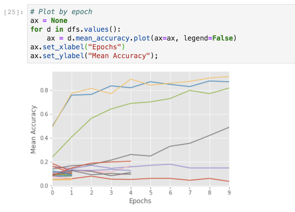
You can run the below in a Jupyter notebook to visualize trial progress.
# Plot by epoch
ax = None  # This plots everything on the same plot
for d in dfs.values():
    ax = d.mean_accuracy.plot(ax=ax, legend=False)
You can also use TensorBoard for visualizing results.
$ tensorboard --logdir {logdir}
Using Search Algorithms in Tune#
In addition to TrialSchedulers, you can further optimize your hyperparameters by using an intelligent search technique like Bayesian Optimization. To do this, you can use a Tune Search Algorithm. Search Algorithms leverage optimization algorithms to intelligently navigate the given hyperparameter space.
Note that each library has a specific way of defining the search space.
from hyperopt import hp
from ray.tune.search.hyperopt import HyperOptSearch

space = {
    "lr": hp.loguniform("lr", -10, -1),
    "momentum": hp.uniform("momentum", 0.1, 0.9),
}

hyperopt_search = HyperOptSearch(space, metric="mean_accuracy", mode="max")

tuner = tune.Tuner(
    train_mnist,
    tune_config=tune.TuneConfig(
        num_samples=10,
        search_alg=hyperopt_search,
    ),
)
results = tuner.fit()

# To enable GPUs, use this instead:
# analysis = tune.run(
#     train_mnist, config=search_space, resources_per_trial={'gpu': 1})
Note
Tune allows you to use some search algorithms in combination with different trial schedulers. See this page for more details.
Evaluating Your Model after Tuning#
You can evaluate the best trained model using the ExperimentAnalysis object to retrieve the best model:
best_result = results.get_best_result("mean_accuracy", mode="max")
with best_result.checkpoint.as_directory() as checkpoint_dir:
    state_dict = torch.load(os.path.join(checkpoint_dir, "model.pth"))

model = ConvNet()
model.load_state_dict(state_dict)
Next Steps#
Check out the Tune tutorials for guides on using Tune with your preferred machine learning library.
Browse our gallery of examples to see how to use Tune with PyTorch, XGBoost, Tensorflow, etc.
Let us know if you ran into issues or have any questions by opening an issue on our GitHub.
To check how your application is doing, you can use the Ray dashboard.