A Simple MapReduce Example with Ray Core#

This example demonstrates how to use Ray for a common distributed computing example––counting word occurrences across multiple documents. The complexity lies in the handling of a large corpus, requiring multiple compute nodes to process the data. The simplicity of implementing MapReduce with Ray is a significant milestone in distributed computing. Many popular big data technologies, such as Hadoop, are built on this programming model, underscoring the impact of using Ray Core.
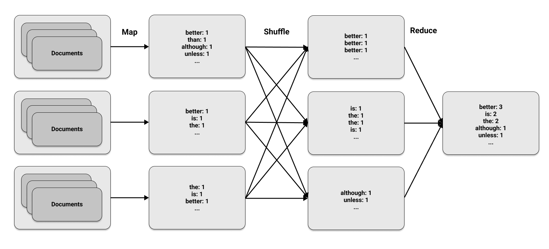
The MapReduce approach has three phases:
Map phase The map phase applies a specified function to transform or map elements within a set of data. It produces key-value pairs: the key represents an element and the value is a metric calculated for that element. To count the number of times each word appears in a document, the map function outputs the pair
(word, 1)every time a word appears, to indicate that it has been found once.Shuffle phase The shuffle phase collects all the outputs from the map phase and organizes them by key. When the same key is found on multiple compute nodes, this phase includes transferring or shuffling data between different nodes. If the map phase produces four occurrences of the pair
(word, 1), the shuffle phase puts all occurrences of the word on the same node.Reduce phase The reduce phase aggregates the elements from the shuffle phase. The total count of each word’s occurrences is the sum of occurrences on each node. For example, four instances of
(word, 1)combine for a final count ofword: 4.
The first and last phases are in the MapReduce name, but the middle phase is equally crucial. These phases appear straightforward, but their power is in running them concurrently on multiple machines. This figure illustrates the three MapReduce phases on a set of documents:
Loading Data#
We use Python to implement the MapReduce algorithm for the word count and Ray to parallelize the computation.
We start by loading some sample data from the Zen of Python, a collection of coding guidelines for the Python community. Access to the Zen of Python, according to Easter egg tradition, is by typing import this in a Python session.
We divide the Zen of Python into three separate “documents” by treating each line as a separate entity
and then splitting the lines into three partitions.
import subprocess
zen_of_python = subprocess.check_output(["python", "-c", "import this"])
corpus = zen_of_python.split()

num_partitions = 3
chunk = len(corpus) // num_partitions
partitions = [
    corpus[i * chunk: (i + 1) * chunk] for i in range(num_partitions)
]
Mapping Data#
To determine the map phase, we require a map function to use on each document.
The output is the pair (word, 1) for every word found in a document.
For basic text documents we load as Python strings, the process is as follows:
def map_function(document):
    for word in document.lower().split():
        yield word, 1
We use the apply_map function on a large collection of documents by marking it as a task in Ray using the @ray.remote decorator.
When we call apply_map, we apply it to three sets of document data (num_partitions=3).
The apply_map function returns three lists, one for each partition so that Ray can rearrange the results of the map phase and distribute them to the appropriate nodes.
import ray

@ray.remote
def apply_map(corpus, num_partitions=3):
    map_results = [list() for _ in range(num_partitions)]
    for document in corpus:
        for result in map_function(document):
            first_letter = result[0].decode("utf-8")[0]
            word_index = ord(first_letter) % num_partitions
            map_results[word_index].append(result)
    return map_results
For text corpora that can be stored on a single machine, the map phase is not necessasry.
However, when the data needs to be divided across multiple nodes, the map phase is useful.
To apply the map phase to the corpus in parallel, we use a remote call on apply_map, similar to the previous examples.
The main difference is that we want three results returned (one for each partition) using the num_returns argument.
map_results = [
    apply_map.options(num_returns=num_partitions)
    .remote(data, num_partitions)
    for data in partitions
]

for i in range(num_partitions):
    mapper_results = ray.get(map_results[i])
    for j, result in enumerate(mapper_results):
        print(f"Mapper {i}, return value {j}: {result[:2]}")
Mapper 0, return value 0: [(b'of', 1), (b'is', 1)]
Mapper 0, return value 1: [(b'python,', 1), (b'peters', 1)]
Mapper 0, return value 2: [(b'the', 1), (b'zen', 1)]
Mapper 1, return value 0: [(b'unless', 1), (b'in', 1)]
Mapper 1, return value 1: [(b'although', 1), (b'practicality', 1)]
Mapper 1, return value 2: [(b'beats', 1), (b'errors', 1)]
Mapper 2, return value 0: [(b'is', 1), (b'is', 1)]
Mapper 2, return value 1: [(b'although', 1), (b'a', 1)]
Mapper 2, return value 2: [(b'better', 1), (b'than', 1)]
This example demonstrates how to collect data on the driver with ray.get. To continue with another task after the mapping phase, you wouldn’t do this. The following section shows how to run all phases together efficiently.
Shuffling and Reducing Data#
The objective for the reduce phase is to transfer all pairs from the j-th return value to the same node.
In the reduce phase we create a dictionary that adds up all word occurrences on each partition:
@ray.remote
def apply_reduce(*results):
    reduce_results = dict()
    for res in results:
        for key, value in res:
            if key not in reduce_results:
                reduce_results[key] = 0
            reduce_results[key] += value

    return reduce_results
We can take the j-th return value from each mapper and send it to the j-th reducer using the following method. Note that this code works for large datasets that don’t fit on one machine because we are passing references to the data using Ray objects rather than the actual data itself. Both the map and reduce phases can run on any Ray cluster and Ray handles the data shuffling.
outputs = []
for i in range(num_partitions):
    outputs.append(
        apply_reduce.remote(*[partition[i] for partition in map_results])
    )

counts = {k: v for output in ray.get(outputs) for k, v in output.items()}

sorted_counts = sorted(counts.items(), key=lambda item: item[1], reverse=True)
for count in sorted_counts:
    print(f"{count[0].decode('utf-8')}: {count[1]}")
is: 10
better: 8
than: 8
the: 6
to: 5
of: 3
although: 3
be: 3
unless: 2
one: 2
if: 2
implementation: 2
idea.: 2
special: 2
should: 2
do: 2
may: 2
a: 2
never: 2
way: 2
explain,: 2
ugly.: 1
implicit.: 1
complex.: 1
complex: 1
complicated.: 1
flat: 1
readability: 1
counts.: 1
cases: 1
rules.: 1
in: 1
face: 1
refuse: 1
one--: 1
only: 1
--obvious: 1
it.: 1
obvious: 1
first: 1
often: 1
*right*: 1
it's: 1
it: 1
idea: 1
--: 1
let's: 1
python,: 1
peters: 1
simple: 1
sparse: 1
dense.: 1
aren't: 1
practicality: 1
purity.: 1
pass: 1
silently.: 1
silenced.: 1
ambiguity,: 1
guess.: 1
and: 1
preferably: 1
at: 1
you're: 1
dutch.: 1
good: 1
are: 1
great: 1
more: 1
zen: 1
by: 1
tim: 1
beautiful: 1
explicit: 1
nested.: 1
enough: 1
break: 1
beats: 1
errors: 1
explicitly: 1
temptation: 1
there: 1
that: 1
not: 1
now: 1
never.: 1
now.: 1
hard: 1
bad: 1
easy: 1
namespaces: 1
honking: 1
those!: 1
For a thorough understanding of scaling MapReduce tasks across multiple nodes using Ray, including memory management, read the blog post on the topic.
Wrapping up#
This MapReduce example demonstrates how flexible Ray’s programming model is. A production-grade MapReduce implementation requires more effort but being able to reproduce common algorithms like this one quickly goes a long way. In the earlier years of MapReduce, around 2010, this paradigm was often the only model available for expressing workloads. With Ray, an entire range of interesting distributed computing patterns are accessible to any intermediate Python programmer.
To learn more about Ray, and Ray Core and particular, see the Ray Core Examples Gallery, or the ML workloads in our Use Case Gallery. This MapReduce example can be found in “Learning Ray”, which contains more examples similar to this one.